Notes on the Finite Element Method 7 Non-linear Advection 9 Time-dependent Viscous Flows

Chapter 8 The Time-dependent Vorticity Equation: Kelvin-Helmholtz Instability

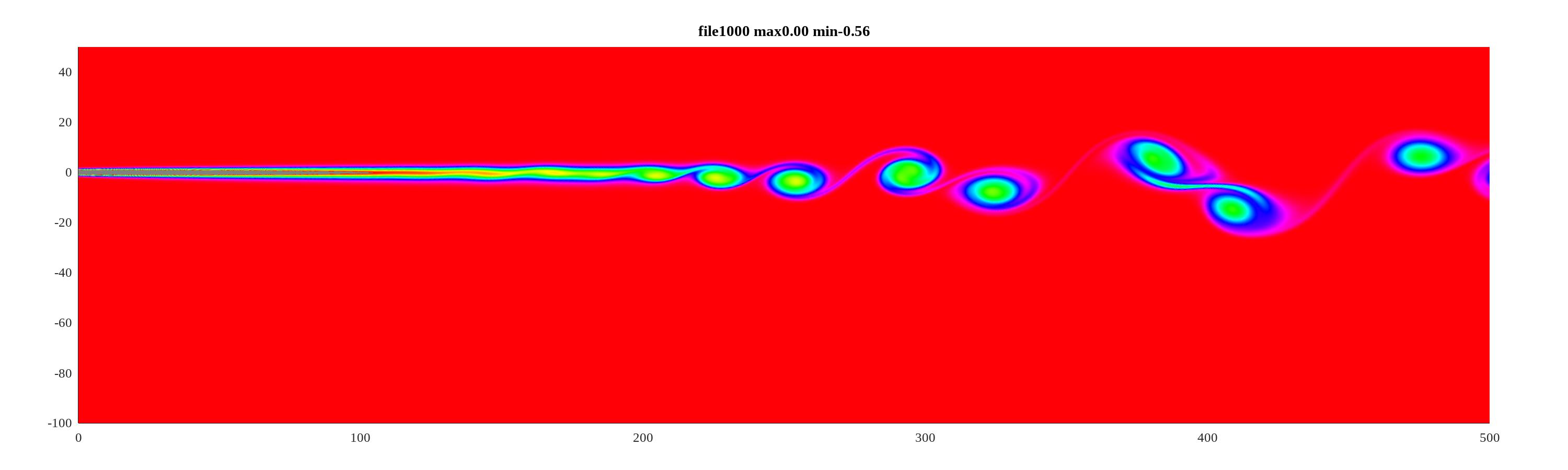
The central feature of shear layers is that they are chronically unstable, and the instabilty lead to first the appearance of Kelvin=Helmholtz billows, followed by interactions between neighboring isolated structures that pair, resulting in new quasi two-dimensional structure that have half the wavenumber and twice the width of the original. These pairing appear to occur repeatedly, until the test section, or the computational domain is filled. Models of two dimensional shear layers are reviewed in the following.

8.1 Analytic Solutions

8.1.1 Equations and Boundary Conditions

Because Shear Layers develop away from solid boundaries, their evolution and growth can be described with the vorticity equation. From a computational perspective, this presents the great advantage that the flow is described by one rather than three dependent variables. In two dimensions the Navier-Stokes equations are:

\bm{u}_{t}+(\bm{u}\cdot\nabla)\bm{u}=-\frac{1}{\rho}\nabla p+\nu\nabla^{2}\bm{u}

(8.1)

Since the divergence of the velocity field is zero, a streamfunction $\psi$ can be defined as:

u=\frac{\partial\psi}{\partial y},\quad v=-\frac{\partial\psi}{\partial x}

(8.2)

In two dimension there is one component of vorticity, which is treated as a scalar:

\omega=\frac{\partial v}{\partial x}-\frac{\partial u}{\partial y}=-\nabla^{2}\psi

(8.3)

With these definitions, taking the curl of equation 8.1 gives an equation for vorticity:

\frac{\partial\omega}{\partial t}+u\frac{\partial\omega}{\partial x}+v\frac{% \partial\omega}{\partial y}=\nu\left(\frac{\partial^{2}\omega}{\partial x^{2}}% +\frac{\partial^{2}\omega}{\partial y^{2}}\right)

(8.4)

There are two different ways to set up the boundary conditions. The simplest is to look at a spatially periodic system where the computational domain extends from $-\pi$ to almost $\pi$ in both directions. The flow field develops much as in the tilted tank that Thorpe used to show the development of the KH instability. These periodic BC make dealing with the spatial discretization and operators with Fourier transforms natural. The second way to cast the problem as in an experiment. At some initial position two streams of different velocities come together, with a small but finite bell-shaped distribution of vorticity near the origin The flow evolves downstream as the shear layer thckness increases, instabilities develop and vortex pairing becomes the principal growth mechanism.

8.1.2 Steady Solutions

The steady form of equation 8.4

\frac{\partial\omega}{\partial t}+u\frac{\partial\omega}{\partial x}+v\frac{% \partial\omega}{\partial y}=\nu\left(\frac{\partial^{2}\omega}{\partial x^{2}}% +\frac{\partial^{2}\omega}{\partial y^{@}}\right)

(8.5)

The boundary layer approximation results in approximating $\omega=-\partial\,u/\partial y$ as well as ignoring the second derivative with respect to $x$ in the parenthesis on the right side of equation 8.5. If the velocities are expressed in terms of the streamfunction, as in equation 8.2, the vorticity equation becomes:

\frac{\partial\psi}{\partial y}\frac{\partial^{2}\psi}{\partial x\partial y}-% \frac{\partial\psi}{\partial x}\frac{\partial^{2}\psi}{\partial y^{2}}=\nu% \frac{\partial^{3}\psi}{\partial y^{3}}

(8.6)

Define similarity variables:

\eta=\frac{y}{2}\sqrt{\frac{U}{\nu x}}\quad\psi=2\sqrt{\nu Ux}f(\eta)

(8.7)

\frac{\partial}{\partial x}=\frac{\partial\eta}{\partial x}\frac{d}{d\eta}=-% \frac{\eta}{2x}\frac{d}{d\eta},\quad\frac{\partial}{\partial y}=\frac{\partial% \eta}{\partial y}\frac{d}{d\eta}=\sqrt{\frac{U}{4\nu x}}\frac{d}{d\eta};

(8.8)

u=\frac{\partial\psi}{\partial y}=U\frac{df}{d\eta},\quad v=-\frac{\partial% \psi}{\partial x}=\sqrt{\frac{U\nu}{x}}\left(\eta\frac{df}{d\eta}-f\right)

(8.9)

\frac{\partial\psi}{\partial y}\frac{\partial^{2}\psi}{\partial x\partial y}=-% \frac{U^{2}}{2x}\eta\frac{df}{d\eta}\frac{d^{2}f}{d\eta^{2}},\quad-\frac{% \partial\psi}{\partial x}\frac{\partial^{2}\psi}{\partial y^{2}}=\frac{U^{2}}{% 2x}\left(\eta\frac{df}{d\eta}-f\right)\frac{d^{2}f}{d\eta^{2}},\quad\frac{% \partial^{3}\psi}{\partial y^{3}}=\frac{U^{2}}{4\nu x}\frac{d^{3}f}{d\eta^{3}}

(8.10)

and the vorticity

\omega=-\frac{\partial^{2}\psi}{\partial x^{2}}-\frac{\partial\psi}{\partial y% ^{2}}=\sqrt{\frac{U\nu}{4\,x^{3}}}\left(f-\eta\frac{df}{d\eta}-\eta^{2}\frac{d% ^{2}f}{d\eta^{2}}\right)-\sqrt{\frac{U^{3}}{4\nu x}}\frac{d^{2}f}{d\eta^{2}}

(8.11)

Introducing these expression into the PDE 8.6 gives:

-\frac{U^{2}}{2x}\eta\frac{df}{d\eta}\frac{d^{2}f}{d\eta^{2}}+\frac{U^{2}}{2x}% \left(\eta\frac{df}{d\eta}-f\right)\frac{d^{2}f}{d\eta^{2}}=\frac{U^{2}}{4x}% \frac{d^{3}f}{d\eta^{3}}

(8.12)

or after dividing by $U^{2}/(2x)$ :

\frac{d^{3}f}{d\eta^{3}}+2\,f\frac{d^{2}f}{d\eta^{2}}=0

(8.13)

If near the origin, the velocity in the upper stream is $u_{1}=U(1+\epsilon)$ and the velocity in the lower stream is $u_{2}=U(1-\epsilon)$ , the boundary conditions become:

\frac{d\,f}{d\eta}\rightarrow 1\pm\epsilon\;\mbox{as}\;\eta\rightarrow\pm\infty

(8.14)

Only two boundary conditions are needed because $f(\eta)$ can have an arbitrary constant added. The BC are:

The linearized solution, valid for small $\epsilon$ , can be recovered by introducing a new independent variable:

f(\eta)=\eta+\epsilon g(\eta)\quad\mbox{or}\quad g(\eta)=\frac{f(\eta)-\eta}{\epsilon}

(8.15)

The problem for $g(\eta)$ is then:

\frac{d^{3}g}{d\eta^{3}}+2\left(\eta+\epsilon g\right)\frac{d^{2}g}{d\eta^{2}}% =0,\quad\left.\frac{dg}{d\eta}\right|_{\eta\rightarrow\pm\infty}=\pm 1

(8.16)

As $\epsilon$ becomes small, the term $\epsilon g$ inside the parenthesis can be neglected. Then if we set $u=dg/d\eta$ , we recover the self-similar version of the heat equation LABEL:eq:C8S1:HeatODE.

Equations 8.16 and 8.14 can be solved numerically with “shooting”, using Newton’s method. The third order ODE 8.16is replced by a sustem of three first order equations:

\frac{df_{1}}{d\eta}=f_{2},\quad\frac{df_{2}}{d\eta}=f_{3},\quad\frac{df_{3}}{% d\eta}=-2f_{1}f_{3}.

(8.17)

Take the $\eta$ axis to range between $-6,~{}6$ and consist of into $n=201$ equispaced points. The boundary condition at $\eta\rightarrow\infty$ is replaced by an initial condition at $\eta=-6$ , taken from the linearized theory:

f_{1}=\eta+\epsilon\left(\eta\mathrm{erf}(\eta)+\frac{\mathrm{e}^{-\eta^{2}}}{% \sqrt{\pi}}\right),\quad f_{2}=1+\epsilon\mathrm{erf}(\eta),\quad f_{3}=2% \epsilon\frac{\mathrm{e}^{-\eta^{2}}}{\sqrt{\pi}}\quad\mbox{where}\quad\eta=-6.

(8.18)

This solution is integrated until $\eta=6$ , and the value of $f_{2}$ is compared with $1+\epsilon\mathrm{erf}(+6)$ . If the difference is small, the solution is adopted, otherwise a new guess at $f_{3}(-6)$ is made, based on the magnitude of the difference $f_{2}(+6)-(1+\epsilon\mathrm{erf}(+6))$ . Convergence is achieved in less than ten iterations.

The functions $f$ calculated with this scheme for different values of $\epsilon$ are illustrated in figure LABEL:Fi:Lock_Soln.

Need some plots here

8.1.3 Instability

Work through Michalke’s solution.

8.2 Finite Element Method

8.2.1 Weak Form

8.2.2 Time Stepping

8.2.3 Results

8.3 Sparse Matrices in Fortran

This is from Run 2 with $\mbox{Re}=100$ , $Volume=10^{-3}$ , $\delta=1.$ , $\epsilon=1/2$ , $dt=0.2$ , write a file every 5 tight cycles, up to 2000 long cycles, so total time covered is $2000$ . Looks like size (xu)=165034,2, also loks like grid file is XTSHL18456.