Notes on the Finite Element Method Notes on the Finite Element Method 2 Tides in a Two-layer Fluid: Solving a System of Equations

Chapter 1 Equilibrium and Co-oscillating Tides

1.1 Tides in a One-dimensional Basin

Equilibrium Tide: Neumann BC.

The equilibrium tide (for a good discussion, read Lamb 6th Ed., 1932, pg .318) describes the perturbation of the surface in response to the gravitational attraction of the moon, for example, if the earth was entirely covered by water. In this case the equilibrium tide would appear as a wave travelling from east to west, with two bulges, one beneath the moon and the other on the opposite side of the earth. On the real earth, the response of the surface is modified by the presence of continents. The equilibrium tide appears as a forcing term in the framework of the linear shallow water (LSW) wave theory. For a one-dimensional basin the mass and momentum conservation equations are:

\frac{\partial\,\eta^{*}}{\partial t^{*}}+\frac{\partial(h^{*}u^{*})}{\partial x% ^{*}}=0,\quad\frac{\partial\,u^{*}}{\partial t^{*}}+g^{*}\frac{\partial(\eta^{% *}-\overline{\eta}^{*})}{\partial x^{*}}=0;\quad u^{*}=0\;\mbox{at}\;x^{*}=\pm L

(1.1)

where variables marked with an asterisk are dimensional. The boundary condition states that there is no velocity at certain locations in the domain (here $x^{*}=\pm L$ ). The equilibrium tide $\overline{\eta}^{*}$ models the forcing resulting from the gravitational attraction between the moon and the earth as a westward (from $+x$ toward $-x$ ) traveling wave:

\overline{\eta}^{*}=\mbox{Re}(\mathrm{e}^{-\mathrm{i}(\sigma^{*}t^{*}+k^{*}x^{% *})})

(1.2)

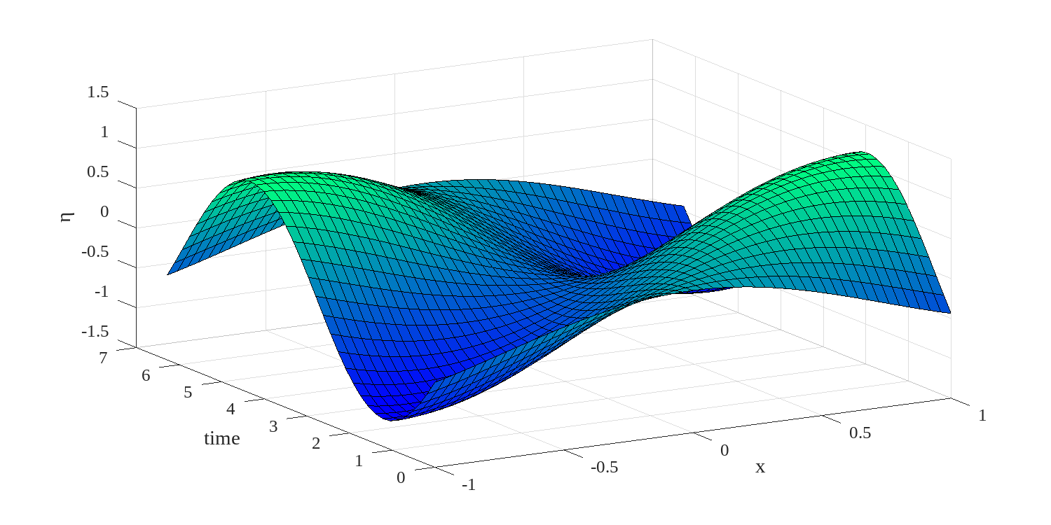
The minus sign in the exponent in equation 1.2 is chosen so that increasing phase corresponds to a lag: if the phase difference between high tide at San Francisco and San Diego is positive, then high tide occurs first at San Diego. The height of the equilibrium tide $\overline{\eta}$ is illustrated in figure 1.1 a a function of time and location. As time increases this wave travels toward $-x$ .

Figure 1.1: Height of the equilibrium tide, $\overline{\eta}$ as a function of time and space. The equilibrium tide is the tide that would exist if the earth was entirely covered by water. The wave crest moves toward $-x$ (toward the west), as time progresses. The wavenumber of the equilibrium tide $k=1$ . Note tha at any time the space mean of $\overline{\eta}$ need not be zero. [C1S1etabar]

After suitable nondimensionalization, with the depth taken to be constant equal to one, and after eliminating the velocity, the sea level is found to obey the wave equation:

\kappa^{2}\frac{\partial^{2}\,\eta}{\partial t^{2}}-\frac{\partial^{2}(\eta-% \overline{\eta})}{\partial x^{2}}=0,\quad\frac{\partial\,(\eta-\overline{\eta}% )}{\partial x}=0\;@\;x=\pm 1

(1.3)

where the new parameter $\kappa=\sigma^{*}L^{*}/\sqrt{g^{*}H^{*}}$ is a measure of the basin length relative to the shallow water wavelength at frequency $\sigma^{*}$ . The governing equation is simplified by introducing the new dependent variable $\eta^{\prime}=\eta-\overline{\eta}$ . The governing equation for the new variable is:

\kappa^{2}\frac{\partial^{2}\,\eta^{\prime}}{\partial t^{2}}-\frac{\partial^{2% }\,\eta^{\prime}}{\partial x^{2}}=0,\quad\frac{\partial\,\eta^{\prime}}{% \partial x}=0\;@\;x=\pm 1

(1.4)

Since there can be no flow through a closed boundary, the second of equations 1.1 implies the gradient of $\eta^{\prime}$ must be zero at such a boundary.

Equation 1.4 is a partial differential equation with two independent variables: time ( $t$ ) and position ( $x$ ). If the forcing and resulting solution are purely periodic, then the solution $\eta^{\prime}$ can be written as:

\eta^{\prime}(x,t)=\mbox{Re}{(N^{\prime}(x)\mathrm{e}^{-\mathrm{i}t})}

(1.5)

and the governing equation for the new dependent variable $N^{\prime}$ is

\frac{d^{2}N^{\prime}}{dx^{2}}+\kappa^{2}N^{\prime}=-\kappa^{2}\mathrm{e}^{-% \mathrm{i}k\,x},\quad\frac{dN^{\prime}}{dx}=0\quad@\quad x=\pm 1.

(1.6)

The partial differential equation has been transformed into a two point boundary value ordinary differential equation. This can be solved exactly by Maxima. The solution for $N^{\prime}$ is:

N^{\prime}=-\frac{\kappa^{2}}{\kappa^{2}-k^{2}}\left[\mathrm{e}^{-\mathrm{i}kx% }+\frac{k}{\kappa}\left(\mathrm{i}\,\frac{\cos{k}\sin{\kappa x}}{\cos{\kappa}}% -\frac{\sin{k}\cos{\kappa x}}{\sin{\kappa}}\right)\right].

(1.7)

So that the complex amplitude and phase of the sea level is:

N=-\frac{k^{2}}{\kappa^{2}-k^{2}}\left[\mathrm{e}^{-\mathrm{i}kx}+\frac{\kappa% }{k}\left(\mathrm{i}\,\frac{\cos{k}\sin{\kappa x}}{\cos{\kappa}}-\frac{\sin{k}% \cos{\kappa x}}{\sin{\kappa}}\right)\right].

(1.8)

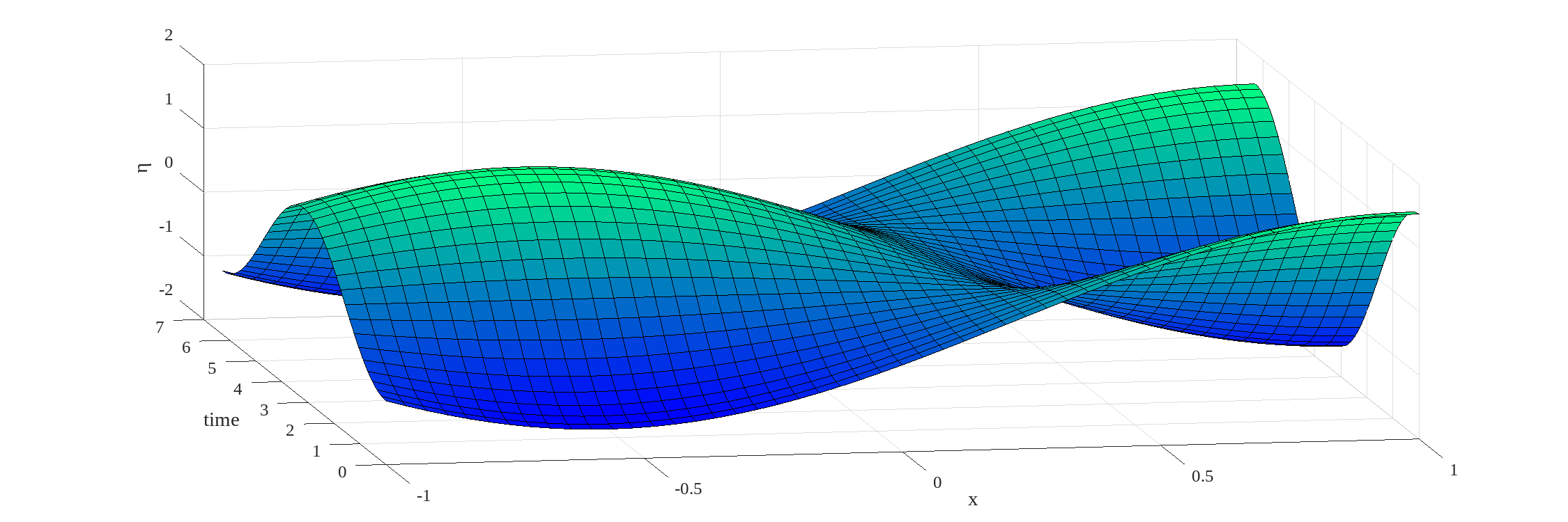
Knowing $N^{\prime}$ , the solution for $\eta^{\prime}$ is given by equation 1.5. The solution $\eta=\eta^{\prime}+\overline{\eta}$ is illustrated in figure 1.2. Even though the forcing (figure 1.1) propagates from right to left, the response appears to consist principally of a standing wave.

It should be noted that the sea level response 1.8 is resonant if the tidal wave number $k$ is equal to $\kappa$ , or if either $\sin{\kappa}$ or $\cos{\kappa}$ are zero. These are the resonances of the basin.

Co-oscillating Tide: Dirichlet BC.

In a much smaller basin, where the equilibrium tide changes little, tides can still occur, forced by the tidal wave propagating in the adjacent ocean vasin. This is called a co-oscillating tide. Examples include tides in marginal seas, estuaries and rivers. These system are governed by equation 1.3, with the tide prescribed (Dirichlet BC) at the end where the estaury opens to the ocean; at the other there is no flux, and the boundary condition is homogeneous Neumann. Looking again for periodic solution, we look for solutions of the form

\eta(x,t)=\mbox{Re}{(N(x)\mathrm{e}^{-\mathrm{i}t})}

(1.9)

The governing equation for $N(x)$ is:

\frac{d^{2}N}{dx^{2}}+\kappa^{2}N=0;\quad\frac{dN}{dx}=0\;@\quad x=1,\quad N=1% \;@\quad x=-1.

(1.10)

The solution is:

N=\frac{\cos{\kappa(1-x)}}{\cos{2\kappa}}.

(1.11)

The solution $\eta(x,t)$ is illustrated in figure 1.3. The sea level disturbance is always maximum at the closed end. The co-oscillating tide can be resonant if $\cos{2\kappa}=0$ .

Sea level response to forcing the ocean tide at one end of
a cooscillating basin. The slope of the surface, — Figure 1.3: Sea level response to forcing the ocean tide at one end of a cooscillating basin. The slope of the surface, $\partial\eta/\partial x$ is always null at the closed end of the basin ( $x=1$ ), consistent with the boundary condition. For this case $\kappa=2$ .

1.2 The Finite Element Method

Reading: Strang pg 247, Whiteley Chap 2

The central concept is to replace an equation such as 1.1 with a system of algebraic equations that, once solved, provides estimates of the solution at a number of points within the domain of interest. While this is basically the same idea as finite differences, the advantage of FEM is that the grid can be unorganized, so that it is ideally suted to finding solutions in real domains. How the differential equation is transformed into a system of algebraic equations is explained in the following.

1.2.1 Weak Form

Given an ODE such as equation 1.6, the first step in the finite element method is to express the equation in the so-called weak form, meaning that al the terms in the equation are multiplied by a test function $\phi(x)$ and integrated over the entire field (here $-1\leq x\leq 1$ ).

\int_{-1}^{1}\!\frac{d^{2}N^{\prime}}{dx^{2}}\phi(x)\,dx+\kappa^{2}\int_{-1}^{% 1}\!\phi(x)\,N^{\prime}\,dx=-\kappa^{2}\int_{-1}^{1}\!\mathrm{e}^{-\mathrm{i}k% \,x}\phi(x)\,dx

(1.12)

The first term can be integrated by parts:

\int_{-1}^{1}\!\frac{d}{dx}\left(\phi\frac{d\,N^{\prime}}{dx}\right)\,dx-\int_% {-1}^{1}\!\frac{d\,N^{\prime}}{dx}\frac{d\,\phi}{dx}\,dx+\kappa^{2}\int_{-1}^{% 1}\!\phi\,N^{\prime}\,dx=-\kappa^{2}\int_{-1}^{1}\!\mathrm{e}^{-\mathrm{i}k\,x% }\phi\,dx

(1.13)

In this case,the divergence theorem states:

\int_{-1}^{1}\!\frac{d}{dx}\left(\phi\frac{d\,N^{\prime}}{dx}\right)\,dx=\left% .\phi\frac{d\,N^{\prime}}{dx}\right|_{-1}^{1}

(1.14)

as long as $\phi$ is a continuous function Equation 1.12 becomes:

-\int_{-1}^{1}\!\frac{d\,N^{\prime}}{dx}\frac{d\,\phi}{dx}\,dx+\kappa^{2}\int_% {-1}^{1}\!N^{\prime}\phi\,dx+\kappa^{2}\int_{-1}^{1}\!\mathrm{e}^{-\mathrm{i}k% \,x}\phi\,dx=\left[\frac{d\,N^{\prime}}{dx}\phi\right]_{-1}^{1}

(1.15)

If the boundary conditions happen to be homogeneous Newmann conditions, as in the equilbrium tide problem, the term on the right side of equation 1.13 contributes nothing, and, after multiplying by $-1$ the weak form is:

\int_{-1}^{1}\!\frac{d\,N^{\prime}}{dx}\frac{d\,\phi}{dx}\,dx-\kappa^{2}\int_{% -1}^{1}\!N^{\prime}\phi\,dx=\kappa^{2}\int_{-1}^{1}\!\mathrm{e}^{-\mathrm{i}k% \,x}\phi\,dx

(1.16)

1.2.2 Discretizing the Domain: the Grid.

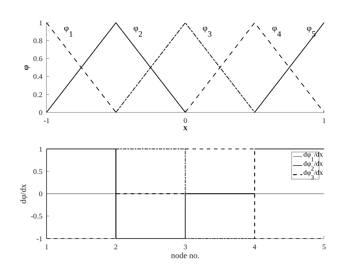
For a one dimensional problem, the simplest grid consists of equispaced nodes along the $x$ -axis, as illustrated in figure 1.4. In this case, the axis extends between $x=\pm 1$ . There are $N=5$ nodes equispaced along the $x$ -axis and $N-1$ segments between the nodes are called elements.

Figure 1.4: One-dimensional piecewise linear functions $\phi_{n}$ (top) and their derivatives . The test function $\phi_{2}$ centerd on node $2$ is shown a solid line. Other Tf are shown as dashed lines. TF derivatives used to compute stiffness are shown in the bottom.

1.2.3 Test and Trial functions

Once the grid is established, the next step is to pick suitable test functions. These same functions will be used in a series expansion of the solution:

\phi_{n}(x)=\sum_{m=1}^{M}\!C_{m,n}x^{m-1},\quad\mbox{where}\quad N^{\prime}(x% )=\sum_{n=1}^{N}\!N^{\prime}_{n}\phi_{n}(x).

(1.17)

The test/trial functions are allways chosen to be polynomials, where $M-1$ is the degree of the polynomial TF, and $N^{\prime}_{n}$ is the value of the solution $N^{\prime}(x)$ at node $x_{n}$ . Each $\phi_{n}$ takes on the value unity at a node, say $x_{n}n$ , and are zero everywhere else: $\phi_{n}(x_{m})=\delta_{m,n}$ .

The central point is that equation 1.13 has to hold for each of these test functions:

\int_{-1}^{1}\!\frac{d\,N^{\prime}}{dx}\frac{d\,\phi_{m}}{dx}\,dx-\kappa^{2}% \int_{-1}^{1}\!N^{\prime}\phi_{m}\,dx=\kappa^{2}\int_{-1}^{1}\!\phi_{m}\mathrm% {e}^{-\mathrm{i}k\,x}\,dx

(1.18)

This is a system of $n x$ equations in $n x$ unknowns. Introduce the expansion 1.17 into the system of equations 1.18:

\sum_{n}\!N^{\prime}_{m}\left[-\int_{-1}^{1}\!\frac{d\,\phi_{m}}{dx}\frac{d\,% \phi_{n}}{dx}\,dx+\kappa^{2}\int_{-1}^{1}\!\phi_{m}\phi_{n}\,dx\right]=-\kappa% ^{2}\int_{-1}^{1}\!\mathrm{e}^{-\mathrm{i}k\,x}\phi_{m}\,dx

(1.19)

Each of the integrals on the left side of equation 1.19 is a matrix element: if, for instance $\mathcal{M}$ (the mass matrix) is a matrix with elements

M_{m,n}=\int_{-1}^{1}\!\phi_{m}(x)\,\phi_{n}(x)\,dx

(1.20)

\mathcal{M}\bm{N^{\prime}}=\sum_{n}\int_{-1}^{1}\!\phi_{m}\phi_{n}\,dx\,N^{% \prime}_{n}

(1.21)

where $\bm{N^{\prime}}$ is a column vector consisting of the solution $N^{\prime}_{n}$ at each node. In matrix notation the system of equations 1.18 is written.

\left[\mathcal{K}-\kappa^{2}\mathcal{M}\right]\,\bm{N^{\prime}}=\bm{F}

(1.22)

where the stiffness matrix elements are

K_{mn}=\int_{-1}^{1}\!\frac{d\,\phi_{m}}{dx}\frac{d\,\phi_{n}}{dx}\,dx

(1.23)

and the load vector elements are

F_{m}=-\kappa^{2}\int_{-1}^{1}\!\mathrm{e}^{-\mathrm{i}k\,x}\phi_{m}\,dx

(1.24)

1.2.4 Assembly

In FEM, the process of determining the values of each element of each matrix is called an assembly. Linear test functions, illustrated in figure 1.4 are written as:

	$\displaystyle\phi_{2}$	$\displaystyle=$	$\displaystyle\frac{x-x_{1}}{\delta x}\quad\mbox{for}\quad x_{1}\leq x\leq x_{2}$		(1.25)
	$\displaystyle\phi_{2}$	$\displaystyle=$	$\displaystyle\frac{x_{3}-x}{\delta x}\quad\mbox{for}\quad x_{2}\leq x\leq x_{3}$

Considering node $2$ , figure 1.4 makes clear that the only place where the integrand of equation 1.20 is non-zero is the interval between nodes $1$ and $3$ . We conclude that most elements of $\mathcal{M}$ (and $\mathcal{K}$ ) are zero. These matrices are sparse. In this example there are just three entries to row $2$ of matrix $\mathcal{M}$ :

M_{2,1}=\frac{\delta x}{6},\quad M_{2,2}=\frac{2\delta x}{3},\quad M_{2,3}=% \frac{\delta x}{6}\quad\mbox{all other}\;M_{2,n}=0.

(1.26)

Entries for each row of each matrix can be found in the same way, with aprticular care exercised for the boundary nodes.

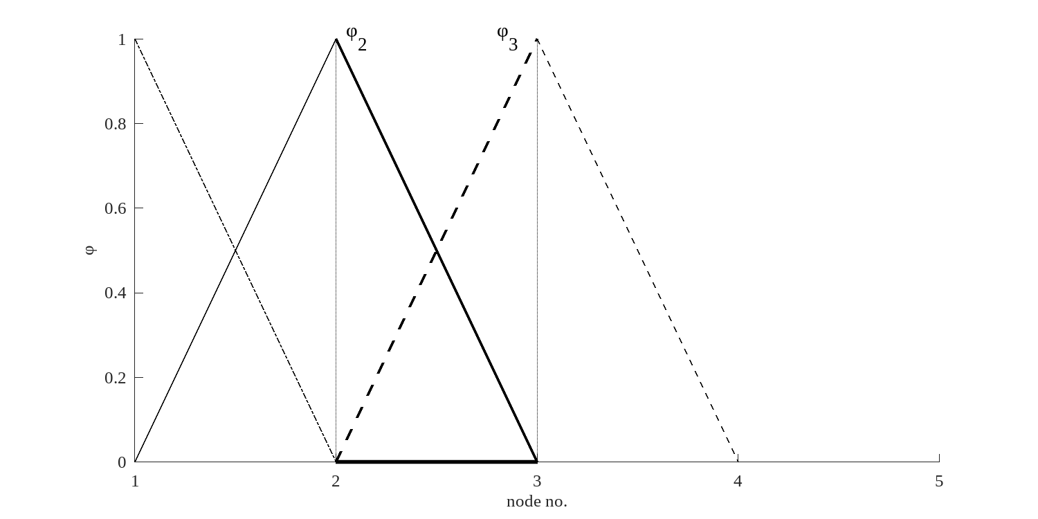
An alternative method, the method that is almost always used in FEM is to assemble each matrix element by element. Consider again element $2$ located between nodes $2$ and $3$ (figure 1.5). There are two pieces of test functions in that element; one sloping down, belongs to the TF associated with the node on the left ( $\phi_{2}$ ); the other, rising, associated with the node on the right ( $\phi_{3}$ ). Element $2$ therefore contributes to $M_{22}$ , $M_{23}$ and to $M_{32}$ , $M_{33}$ . These four contributions define an Element Matrix.

\mathcal{M}e=\begin{bmatrix}Me_{22}&Me_{23}\\ Me_{32}&Me_{33}\end{bmatrix}=\frac{\delta x}{6}\begin{bmatrix}2&1\\ 1&2\end{bmatrix}

(1.27)

The numerical values are obtained by evaluating the integrals in equation 1.20. A stiffness element matrix can be defined and eveluated in the same way:

\mathcal{K}e=\frac{1}{\delta x}\begin{bmatrix}1&-1\\ -1&1\end{bmatrix}

(1.28)

The next step is to combine the element matrices to form the global matrices. For the five node, four element grid illustrated in figure 1.4, there are four steps. The constitution of $\mathcal{M}$ after each step is shown in equation 1.29:

\mathcal{M}=\frac{\delta x}{6}\begin{bmatrix}2&1&0&0&0\\ 1&2&0&0&0\\ 0&0&0&0&0\\ 0&0&0&0&0\\ 0&0&0&0&0\end{bmatrix};\frac{\delta}{6}\begin{bmatrix}2&1&0&0&0\\ 1&4&1&0&0\\ 0&1&2&0&0\\ 0&0&0&0&0\\ 0&0&0&0&0\end{bmatrix};\frac{\delta}{6}\begin{bmatrix}2&1&0&0&0\\ 1&4&1&0&0\\ 0&1&4&1&0\\ 0&0&1&2&0\\ 0&0&0&0&0\end{bmatrix};\frac{\delta}{6}\begin{bmatrix}2&1&0&0&0\\ 1&4&1&0&0\\ 0&1&4&1&0\\ 0&0&1&4&1\\ 0&0&0&1&2\end{bmatrix}.

(1.29)

In the first step, matrix $\mathcal{M}e$ is added to the upper left corner of $\mathcal{M}$ . During the second step matrix $\mathcal{M}e$ is added to the second and third rows, as well as second and third columns of $\mathcal{M}$ , with the result that $M_{22}$ reaches the value $2\delta x/3$ . After the elemnt matrix for the last element ( $4$ ) has been added, $\mathcal{M}$ is complete.

Following the same procedure, the stiffness matrix assembles as:

\mathcal{K}=\frac{1}{\delta x}\begin{bmatrix}1&-1&0&0&0\\ -1&2&-1&0&0\\ 0&-1&2&-1&0\\ 0&0&-1&2&-1\\ 0&0&0&-1&1\end{bmatrix}

(1.30)

There are several ways to assemble the forcing vector $\bm{F}$ . The simplest is to assume that the forcing, in this case $\mathrm{e}^{-\mathrm{i}k\,x}$ , does not change much over an element. This is surely a poor approximation with a five element matrix, and alternative methods are discussed in detail in section 1.3. For now write the element vector:

\bm{Fe}=\frac{\delta x}{2}\begin{bmatrix}1\\ 1\end{bmatrix}

(1.31)

If the forcing function was constant, each element would contribute $\bm{Fe}$ to the global forcing vector. In this case, the global forcing vector is:

\bm{F}=-\frac{\kappa^{2}\,dx}{2}\begin{bmatrix}1\\ 2\\ 2\\ 2\\ 1\end{bmatrix}\mathrm{e}^{-\mathrm{i}\,k\,\bm{x}}

(1.32)

1.2.5 Solving the linear system

Once the matrices and the forcing vector have been assembled. the solution is found by solving the linear system 1.22. Make sure to use a sparse method. It is always a bad idea to attempt to solve the system by inverting the global matrix, because the inverse of a sparse matrix is not necessarily sparse.

The solution is found with script 1. The FEM solution agrees well with the analytic solution 1.7. The error, defined as the maximum value of the absolute value of the difference between the exact solution and the FEM solution is listed in table 1.1 as a function of the number of nodes $N$ .

M	11	21	51	101	201	501	1001
Linear TF	$3.2\;10^{-2}$	$7.8\;10^{-3}$	$1.3\;10^{-3}$	$3.1\;10^{-4}$	$7.8\;10^{-5}$	$1.3\;10^{-5}$	$3.1\;10^{-6}$
Quadratic TF	$4.6\;10^{-2}$	$1.2\;10^{-2}$	$1.9\;10^{-3}$	$4.8\;10^{-4}$	$1.2\;10^{-4}$	$1.9\;10^{-5}$	$4.8\;10^{-6}$
Quad TF+Quadrature	$1.2\;10^{-3}$	$7.5\;10^{-5}$	$2.0\;10^{-6}$	$1.2\;10^{-7}$	$7.6\;10^{-9}$	$1.7\;10^{-10}$	$5.0\;10^{-11}$

Table 1.1: Error between FEM and exact solutions for the equilibrium tide in a closed basin, as a function of grid density

M

Table 1.1 leads to the conclusion that with linear TF, the error decreases as the square of the number of nodes.

1.3 Bells and Whistles

1.3.1 Choice of Test Functions

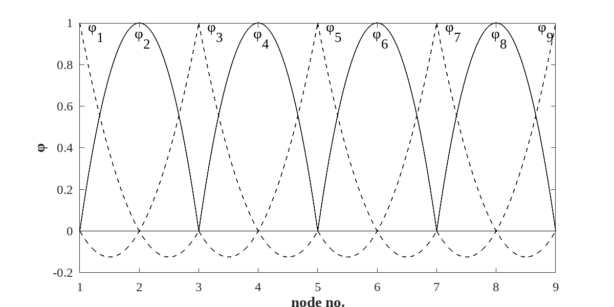
In principle there are an infinite number of polynomials that can be used as test functions. For example the linear TF given in equation 1.25 can be relaced by quadratic functions (or cubics, etc…). Since three constants are needed to define a second order polynomial, an extra node is added to each element. If, as in the case of linear test functions (figue 1.6) the axis extends from $-1\leq x\leq 1$ with four elements, there will be $M=9$ nodes. The grid and quadratic test functions are illustrated in figure

Figure 1.6: One-dimensional piecewise quadratic functions $\phi_{n}$ on a four element domain with $9$ nodes. Each test function is $1$ at the corresponding node and zero at all other nodes.

Consider element $n$ which extends between nodes $2n-1$ and $2n+1$ . The canonical variable is:

\tilde{x}=\frac{x-x_{2n-1}}{x_{2n+1}-x_{2n-1}},\quad 0\leq X\leq 1

(1.33)

The ends of the element ends are located at $\tilde{x}=0,1$ , and the midpoint is located at $\tilde{x}=1/2$ . The three TF that are non-zero in this element are given by:

$\displaystyle\phi_{n-1}$	$\displaystyle=$	$\displaystyle 2\tilde{x}^{2}-3\tilde{x}+1$
$\displaystyle\phi_{n}$	$\displaystyle=$	$\displaystyle 4\tilde{x}-4\tilde{x}^{2}$	(1.34)
$\displaystyle\phi_{n+1}$	$\displaystyle=$	$\displaystyle 2\tilde{x}^{2}-\tilde{x}$

The quadratic test functions are illustrated in figure 1.6.

The mass, stiffness and load contribution made by each element to the global matrices are:

\mathcal{M}e=\frac{\delta x}{30}\begin{bmatrix}4&2&-1\\ 2&16&2\\ -1&2&4\end{bmatrix}\quad\mathcal{K}e=\frac{1}{3\delta x}\begin{bmatrix}7&-8&1% \\ -8&16&-8\\ 1&-8&7\end{bmatrix}\quad\bm{F}e=\frac{\delta x}{6}\begin{bmatrix}1\\ 4\\ 1\end{bmatrix}

(1.35)

Assembly still proceeds element by element. The condition of the mass matrix $\mathcal{M}$ after the contributions from elements 1 and 2 is

\mathcal{M}=\frac{\delta x}{30}\begin{bmatrix}4&2&-1&0&0&0&0&0&0\\ 2&16&2&0&0&0&0&0&0\\ -1&2&4&0&0&0&0&0&0\\ 0&0&0&0&0&0&0&0&0\\ 0&0&0&0&0&0&0&0&0\\ 0&0&0&0&0&0&0&0&0\\ 0&0&0&0&0&0&0&0&0\\ 0&0&0&0&0&0&0&0&0\\ 0&0&0&0&0&0&0&0&0\\ \end{bmatrix};\frac{\delta x}{30}\begin{bmatrix}4&2&-1&0&0&0&0&0&0\\ 2&16&2&0&0&0&0&0&0\\ -1&2&8&2&-1&0&0&0&0\\ 0&0&2&16&2&0&0&0&0&\\ 0&0&-1&2&4&0&0&0&0\\ 0&0&0&0&0&0&0&0&0\\ 0&0&0&0&0&0&0&0&0\\ 0&0&0&0&0&0&0&0&0\\ 0&0&0&0&0&0&0&0&0\\ \end{bmatrix}.

(1.36)

The norm of the difference between the FEM solution with quadratic TF and the analytic solution is shown in table 1.1. The errors is found to be slightly larger than the error associated with linear TF

1.3.2 Quadrature

Thi last result is surprising, since errors associated with higher order polynomiala ought to be smaller. This motivates evaluatinng the forcing function more carefully. One way to improve the solution given above is to use quadrature to evaluate the integral in equation 1.24. For quadrature, the integrand is evaluated at a number of points in the interval $0\leq x\leq 1$ . The integral is then approximated by a weighted sum of the three values. In this case a three point quadrature scheme for the one-dimensional integral over an element of length $\delta x$ is:

Fe_{m}=-\kappa^{2}\,dx\sum_{q=1}^{3}\!w_{q}\mathrm{e}^{-\mathrm{i}\,k\,\tilde{% x}_{q}}\phi_{m}(x_{q})\quad\mbox{where}\quad\tilde{x}_{q}=x_{2n-1}+\delta x\,x% _{q}.

(1.37)

where $w_{q}$ and $x_{q}$ represent the quadrature weights and quadrature points for any given scheme.

Table 1.1 shows marked reduction in the error between the FEM solution and the analytical solution, when both quadratic TF are used and the load integral is estimated using quadrature. In that case, the error decreases as the fourth power of the number of nodes.

1.3.3 Dirichlet Boundary Conditions

In the cooscillating tide problem there is no forcing term on the right side of the governing equation 1.6. Instead the problem is forced by the Dirichlet condition at the boundary between estaury and ocean. Using matrix notation the weak form is:

\mathcal{L}\,\bm{N}=\left[\kappa^{2}\mathcal{M}-\mathcal{K}\right]\,\bm{N}=0% \quad\mbox{with}\quad N_{1}=1.

(1.38)

where $\mathcal{L}=\kappa^{2}\mathcal{M}-\mathcal{K}$ . If the full domain consists of $M$ nodes, only $M-1$ of these are unknown since the value $N_{1}$ is given. For example in the case where the $x$ -axis is divided into four elements with $5$ nodes, if $\mathcal{L}=\kappa^{2}\mathcal{M}-\mathcal{K}$ , equation 1.38 is:

\begin{bmatrix}L_{11}&L_{12}&L_{13}&L_{14}&L_{15}\\ L_{21}&L_{22}&L_{23}&L_{24}&L_{25}\\ L_{31}&L_{32}&L_{33}&L_{34}&L_{35}\\ L_{41}&L_{42}&L_{43}&L_{44}&L_{45}\\ L_{51}&L_{52}&L_{53}&L_{54}&L_{55}\end{bmatrix}\begin{bmatrix}1\\ N_{2}\\ N_{3}\\ N_{4}\\ N_{5}\end{bmatrix}=0

(1.39)

The first row of equation 1.39 is irrelevant since $N_{1}$ is already known. In the remaing rows the contributions from known elements is separated from the unknown part:

\widehat{\mathcal{L}}N_{1}+\widetilde{\mathcal{L}}\begin{bmatrix}N_{2}\\ N_{3}\\ N_{4}\\ N_{5}\end{bmatrix}=0

(1.40)

where $\widehat{\mathcal{L}}$ is a column vector, and $\widetilde{\mathcal{L}}$ is a $4\times 4$ matrix:

\widehat{\mathcal{L}}=\begin{bmatrix}L_{21}\\ L_{31}\\ L_{41}\\ L_{51}\end{bmatrix};\quad\widetilde{\mathcal{L}}=\begin{bmatrix}L_{22}&L_{23}&% L_{24}&L_{25}\\ L_{32}&L_{33}&L_{34}&L_{35}\\ L_{42}&L_{43}&L_{44}&L_{45}\\ L_{52}&L_{53}&L_{54}&L_{55}\end{bmatrix}

(1.41)

Equation 1.42 can now be written:

\widetilde{\mathcal{L}}\begin{bmatrix}N_{2}\\ N_{3}\\ N_{4}\\ N_{5}\end{bmatrix}=-\widehat{\mathcal{L}}N_{1}

(1.42)

where the known terms appear on the right. The number of simultaneous equations is reduced by the number of Dirichlet points.

Errors using linear and quadratic test functions for different grid sizes are compared in table 1.2. This shows that errors associated with quadratic TF are much smaller than those with linear TF. As the order of the polynomial used as a test function increases, the accuracy of the solution increases.

nx	11	21	51	101	201	501	1001
Linear TF	$5.1\;10^{-2}$	$1.3\;10^{-2}$	$2.1\;10^{-3}$	$5.5\;10^{-4}$	$1.4\;10^{-4}$	$2.2\;10^{-5}$	$5.5\;10^{-6}$
Quadratic TF	$2.5\;10^{-3}$	$1.5\;10^{-4}$	$4.2\;10^{-6}$	$2.6\;10^{-7}$	$1.6\;10^{-8}$	$4.0\;10^{-10}$	$1.8\;10^{-11}$

Table 1.2: Error between FEM and exact solutions for the cooscillating tide in a semiclosed basin, as a function of

n x

, the number of points on the grid.

Exercises

1.

Write a script that solves the same problem as script 1 from scratch (no need to worry about quadrature for this).
2.

Solve Helmholtz’ equation for different values of $\kappa$ and $k$ . When does the code not work?
3.

Modify the script so that it handles steep changes in depth. For example $|x|\leq 1/2,~{}h=1;~{}~{}1/2<|x|\leq 1,~{}h=1/10$ .
4.

Modify this new script to work with quadratic TF.

Scripts

Octave: Analytic Solution to the Forced Wave Equation

⬇

clear;

%%ID Chap 1 S1; Analytic solution to equilibrium tide kappa=2;k=1;

%Grids

nx=51;x=linspace(-1,1,nx);x=transpose(x);dx=diff(x(1:2));

nt=37;t=linspace(0,2*pi,nt);

kappa=2;k=1;

ck=cos(k);sk=sin(k);cs=cos(kappa);ss=sin(kappa);

step=k*exp(-i*k*x)+kappa*(i*ck*sin(kappa*x)/cs-sk*cos(kappa*x)/ss);

cons=k/(k^2-kappa^2);N=cons*step;

for kt=1:nt

equileta(kt,:)=real(N*exp(-i*t(kt)));

endfor

set(gcf,’position’,[20,1000,1500,500]);clf

surf(x,t,equileta);colormap(winter);

view([-30.,30.]);

xlabel(’x’,’fontsize’,14)

ylabel(’time’,’fontsize’,14)

zlabel(’\eta’,’fontsize’,14)

set(gcf,’paperpositionmode’,’manual’,’paperposition’,[0.25␣0.25␣10␣5])

print␣-dpng␣../../words/figs/C1/C1S1equileta.png

Octave: FEM Solution to the Forced Wave Equation

⬇

clear;

%%ID Chap 1 S3; cmp ana FEM homo Nmn BC;quadTF;kappa=2;k=1;nx=101

%%ID evaluate forcing using quadrature.

%% compare analytic and quad fem solutions to forced Hemholtz with homo Neumann

function N = Nexact (x,kappa,k)

%% This is N, not N’, or anything else: N=N’+Nbar

ck=cos(k);sk=sin(k);cs=cos(kappa);ss=sin(kappa);

step=k*exp(-i*k*x)+kappa*(i*ck*sin(kappa*x)/cs-sk*cos(kappa*x)/ss);

cons=k/(k^2-kappa^2);N=cons*step;

endfunction

%% Problem Param

kappa=2;k=1;

npts=[11,21,51,101,201,501,1001];

for kn=1:7

np=npts(kn);xp=transpose(linspace(-1,1,np));dx=2*diff(xp(1:2));

tp=[(1:2:np-2)’,(3:2:np)’];ne=size(tp,1);

%%␣␣FEM␣quadratic␣TF

Me=dx*[4,2,-1;2,16,2;,-1,2,4]/30;

Ke=[7,-8,1;-8,16,-8;1,-8,7]/3/dx;

M=K=sparse(np,np);F=zeros(np,1);

%%␣here␣load␣by␣quadrature

QuadWeights␣=␣[5/18,4/9,5/18];

QuadPoints␣=␣[0.5*(1-sqrt(0.6)),0.5,0.5*(1+sqrt(0.6))]␣;

for␣ke=1:ne

␣␣nodes=[tp(ke,1):tp(ke,2)];

␣␣M(nodes,nodes)=M(nodes,nodes)+Me;

␣␣K(nodes,nodes)=K(nodes,nodes)+Ke;

␣␣Fe=zeros(3,1);

␣␣for␣kquad=1:3

␣␣␣␣X␣=␣QuadPoints(kquad);W=QuadWeights(kquad);

␣␣␣␣phi=[2*X^2-3*X+1,4*X-4*X^2,2*X^2-X];

␣␣␣␣for␣km=1:3

␣␣␣␣␣␣Fe(km,1)=Fe(km,1)+dx*W*kappa^2*exp(-i*k*(xp(nodes(1))+dx*X))*phi(km);

␣␣␣␣endfor

␣␣endfor

␣␣F(nodes,1)=F(nodes,1)+Fe;

endfor

%%␣Here␣I␣am␣comparing␣N’

X=(K-kappa^2*M)\F;##␣this␣is␣X

Xact=Nexact(xp,kappa,k)-exp(-i*k*xp);

Err=norm(X-Xact,’Inf’)

endfor