Notes on the Finite Element Method 1 Equilibrium and Co-oscillating Tides 3 Time-dependent Waves and Burgers’ Equation

Chapter 2 Tides in a Two-layer Fluid: Solving a System of Equations

It is often the case that the partial differential equations that govern flows are stated in term of multiple dependent variables. A two-layer hydrostatic fluid, where displacements of both the free surface and the inteface are sought, provides an example of how the FEM procedure can be adapted to determine the solutions.

2.1 The Problem

The one-dimesional basin described in the previous chapter is now filled with two fluids of different density: the top layer, of constant thickness $\hbar$ , sits on top of a heavier layer of variable height (figure 2.1). The maximum depth beneath the surface is taken to be one.

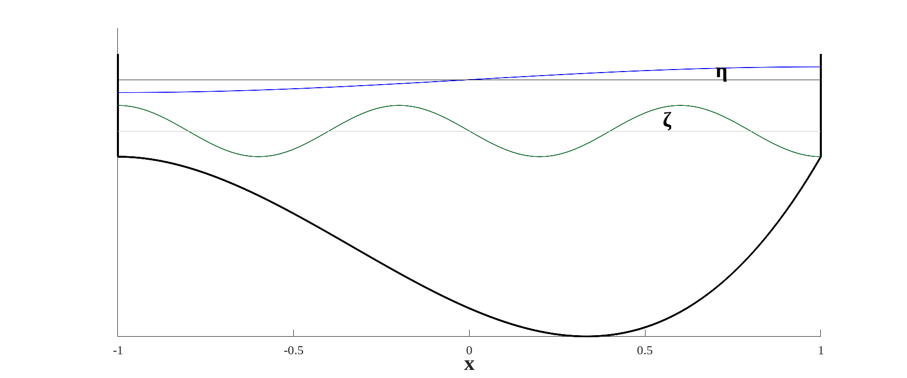
As before the free surface displacement from the mean sea level is $\eta(x,t)$ ; the displacement of the interface from $z=-\hbar$ is $\zeta$ . The velocity in the upper layer is $u_{1}(x,t)$ . In the lower layer the velocity is $u_{2}(x,t)$ . the density anomaly between the two layers is $\rho=2(\rho_{2}-\rho_{1})/(\rho_{1}+\rho_{2})$ .

2.1.1 Equations and BC

After suitable non-dimensionalization, conserving mass in each layer gives the two equations:

\frac{\partial(\eta-\zeta)}{\partial t}+\hbar\frac{\partial\,u_{1}}{\partial x% }=0,\quad\frac{\partial\zeta}{\partial t}+(1-\hbar)\frac{\partial\,u_{2}}{% \partial x}=0,

(2.1)

and the momentum equations for each layer are:

\frac{\partial\,u_{1}}{\partial t}+\frac{\partial\,\eta}{\partial x}=\frac{% \partial\,\overline{\eta}}{\partial x},\quad\frac{\partial\,u_{2}}{\partial t}% +\frac{\partial(\eta-\overline{\eta})}{\partial x}+\rho\frac{\partial\,\zeta}{% \partial x}=0

(2.2)

Look for periodic solutions of the form:

	$\displaystyle\eta(x,y,t)=\Re{N(x,y)e^{-i\,t}},\quad\zeta(x,y,t)=\Re{I(x,y)e^{-% i\,t}}$		(2.3)
	$\displaystyle u_{1}(x,y,t)=\Re{U_{1}(x,y)e^{-i\,t}},\quad u_{2}(x,y,t)=\Re{U_{% 2}(x,y)e^{-i\,t}}.$		(2.4)

Momentum conservation in each layer determines the transport in terms of pressure gradient:

U_{1}=-\frac{\mathrm{i}\hbar}{\kappa^{2}}\frac{d\,N^{\prime}}{dx};\quad U_{2}=% -\frac{\mathrm{i}(h-\hbar)}{\kappa^{2}}\frac{d(N^{\prime}+\rho\,I)}{dx};

(2.5)

where $N^{\prime}=N-\overline{N}$ is the departure of the sea level from the forcing, taken to be an equilibrium tide. The mass conservation relations in each layer are:

\frac{d\,U_{1}}{dx}-\mathrm{i}(N-I)=0;\quad\frac{d\,U_{2}}{dx}-\mathrm{i}\,I=0.

(2.6)

Substituting relations 2.5 into equations 2.6 yields a system of nonhomogeneous ordinary differential equations for the dependent variables $N^{\prime}$ and $I$ :

	$\displaystyle\hbar\frac{d^{2}N^{\prime}}{dx^{2}}+\kappa^{2}(N^{\prime}-I)=-% \kappa^{2}\overline{N},$		(2.7)
	$\displaystyle\frac{d}{dx}\left[(h-\hbar)\frac{d(N^{\prime}+\rho\,I)}{dx}\right% ]+\kappa^{2}I=0.$

The boundary conditions require that the transports ( $\hbar U_{1}$ and $(1-\hbar)U_{2}$ ) be zero at each extremity:

\frac{d\,N^{\prime}}{dx}=0;\quad\frac{d\,I}{dx}=0\quad\mbox{at}\quad x=\pm 1.

(2.8)

2.1.2 Analytic Solution

Solve the first of equations 2.7 for $I$ :

I=N^{\prime}+\overline{N}+\frac{\hbar}{\kappa^{2}}\frac{d^{2}N^{\prime}}{dx^{2}}

(2.9)

Introduce this expression into the second of equations 2.7:

\frac{d}{dx}\left\{(h-\hbar)\frac{d}{dx}\left[N^{\prime}+\rho\left(N^{\prime}+% \overline{N}+\frac{\hbar}{\kappa^{2}}\frac{d^{2}N^{\prime}}{dx^{2}}\right)% \right]\right\}+\kappa^{2}\left(N^{\prime}+\overline{N}+\frac{\hbar}{\kappa^{2% }}\frac{d^{2}N^{\prime}}{dx^{2}}\right)=0.

(2.10)

or, after gathering terms:

\rho\hbar\frac{d}{dx}\left[(h-\hbar)\frac{d^{3}N^{\prime}}{dx^{3}}\right]+% \kappa^{2}\frac{d}{dx}\left\{\left[h+\rho\,(h-\hbar)\right]\frac{dN^{\prime}}{% dx}\right\}+\kappa^{4}N^{\prime}=-\kappa^{2}\left\{\kappa^{2}\overline{N}+\rho% \frac{d}{dx}\left[(h-\hbar)\frac{d\overline{N}}{dx}\right]\right\}

(2.11)

The boundary conditions are:

\frac{d\,N^{\prime}}{dx}=0;\quad\frac{d^{3}\,N^{\prime}}{dx^{3}}=-\frac{\kappa% ^{2}}{\hbar}\frac{d\overline{N}}{dx}\;\mbox{at}\;x=\pm 1;

(2.12)

and the forcing is taken as a wave travelling from right to left:

\overline{N}=\mathrm{e}^{(-\mathrm{i}k\,x)}

(2.13)

The solution to equation 2.11 can be written as the sum of a particular solution and a homogeneous solution:

N^{\prime}=N^{p}+N^{h}

(2.14)

The equation governing the particular solution $N^{p}$ is:

\rho\hbar(h-\hbar)\frac{d^{4}N^{p}}{dx^{4}}+\kappa^{2}\left(h+\rho\,(h-\hbar)% \right)\frac{d^{2}N^{p}}{dx^{2}}+\kappa^{4}N^{p}=\kappa^{2}(\rho(h-\hbar)k^{2}% -\kappa^{2})e^{-i\,kx}

(2.15)

For the particular solution, try $N^{p}=A\mathrm{e}^{(-\mathrm{i}k\,x)}$ , plug into 2.15:

A\left(\rho\hbar(h-\hbar)k^{4}-\kappa^{2}\left(h+\rho\,(h-\hbar)\right)k^{2}+% \kappa^{4}\right)=\kappa^{2}(\rho(h-\hbar)k^{2}-\kappa^{2})

(2.16)

This can be solved for $A$ :

A=\frac{\kappa^{2}(\rho(h-\hbar)k^{2}-\kappa^{2})}{\rho\hbar(h-\hbar)k^{4}-% \kappa^{2}k^{2}\left(h+\rho\,(h-\hbar)\right)+\kappa^{4}}

(2.17)

Note that if $\rho\hbar(h-\hbar)\ll 1$ , $A=\kappa^{2}/(k^{2}-\kappa^{2})$ , usually less than one (since $k<\kappa$ ).

For the homogeneous part, $N^{h}$ is the solution of:

\rho\hbar(h-\hbar)\frac{d^{4}N^{h}}{dx^{4}}+\kappa^{2}\left(h+\rho\,(h-\hbar)% \right)\frac{d^{2}N^{h}}{dx^{2}}+\kappa^{4}N^{h}=0

(2.18)

If solutions are sought with wavenumber $k$ , equation 2.18 gives a fourth order algebraic equation for $k$ :

\rho\hbar(h-\hbar)k^{4}-\kappa^{2}\left(h+\rho\,(h-\hbar)\right)k^{2}+\kappa^{% 4}=0

(2.19)

with solutions:

\begin{split}\displaystyle k^{2}=\kappa^{2}\frac{h+\rho(h-\hbar)-\sqrt{h^{2}+2% \rho(h-\hbar)(1-2\hbar)+\rho^{2}(h-\hbar)^{2}}}{2\rho\hbar(h-\hbar)},\\ \displaystyle k^{\prime 2}=\kappa^{2}\frac{h+\rho(h-\hbar)+\sqrt{h^{2}+2\rho(h% -\hbar)(1-2\hbar)+\rho^{2}(h-\hbar)^{2}}}{2\rho\hbar(h-\hbar)};\end{split}

(2.20)

A general solution to equation 2.18 is:

N^{h}=S\sin{kx}+C\cos{kx}+S^{\prime}\sin{k^{\prime}x}+C^{\prime}\cos{k^{\prime% }x}

(2.21)

where the four constants $S$ , $C$ , $S^{\prime}$ , $C^{\prime}$ are evaluated by enforcing the boundary conditions on equation 2.18:

\frac{d\,N^{h}}{dx}=-\frac{d\,N^{p}}{dx}\;,\frac{d^{3}\,N^{h}}{dx^{3}}=-\frac{% \kappa^{2}}{\hbar}\frac{d\overline{N}}{dx}-\frac{d^{3}\,N^{p}}{dx^{3}}\;\mbox{% at}\;x=0,1;

(2.22)

The constants are found to be:

\begin{split}\displaystyle S=-\frac{i\,k\,\cos k\,\left[A\hbar(k^{2}-k^{\prime 2% })-\kappa^{2}\right]}{\hbar\,k\,\cos k\,\left(k^{\prime 2}-k^{2}\right)},&% \displaystyle C=\frac{k\,\sin k\,\left[A\hbar(k^{2}-k^{\prime 2})-\kappa^{2}% \right]}{\hbar\,k\,\sin k\,\left(k^{\prime 2}-k^{2}\right)},\\ \displaystyle S^{\prime}=\frac{i\,k\,\cos k\,\left[A\hbar(k^{2}-k^{2})-\kappa^% {2}\right]}{\hbar\,k^{\prime}\,\cos k^{\prime}\,\left(k^{\prime 2}-k^{2}\right% )},&\displaystyle C^{\prime}=-\frac{k\,\sin k\,\left[A\hbar(k^{2}-k^{2})-% \kappa^{2}\right]}{\hbar\,k^{\prime}\,\sin k^{\prime}\,\left(k^{\prime 2}-k^{2% }\right)}.\end{split}

(2.23)

Any Computer Algebra System (CAS) can really help solving systems of equations such as above. I use Maxima, but Mathematica and Maple are quite popular. The solutions are resonant if either $k$ or $k^{\prime}$ are equal to $n\pi$ for $n=1,2,\cdots$ . Otherwise the constants $S^{\prime}$ and $C^{\prime}$ are usually small, as they depend on $k^{\prime-3}$ . The solution is:

N=A\mathrm{e}^{-\mathrm{i}kx}+S\sin{kx}+C\cos{kx}+S^{\prime}\sin{k^{\prime}x}+% C^{\prime}\cos{k^{\prime}x}+\overline{N},\quad I=N+\frac{\hbar}{\kappa^{2}}% \frac{d^{2}N^{\prime}}{dx^{2}}

(2.24)

with $A$ given by equation 2.17.

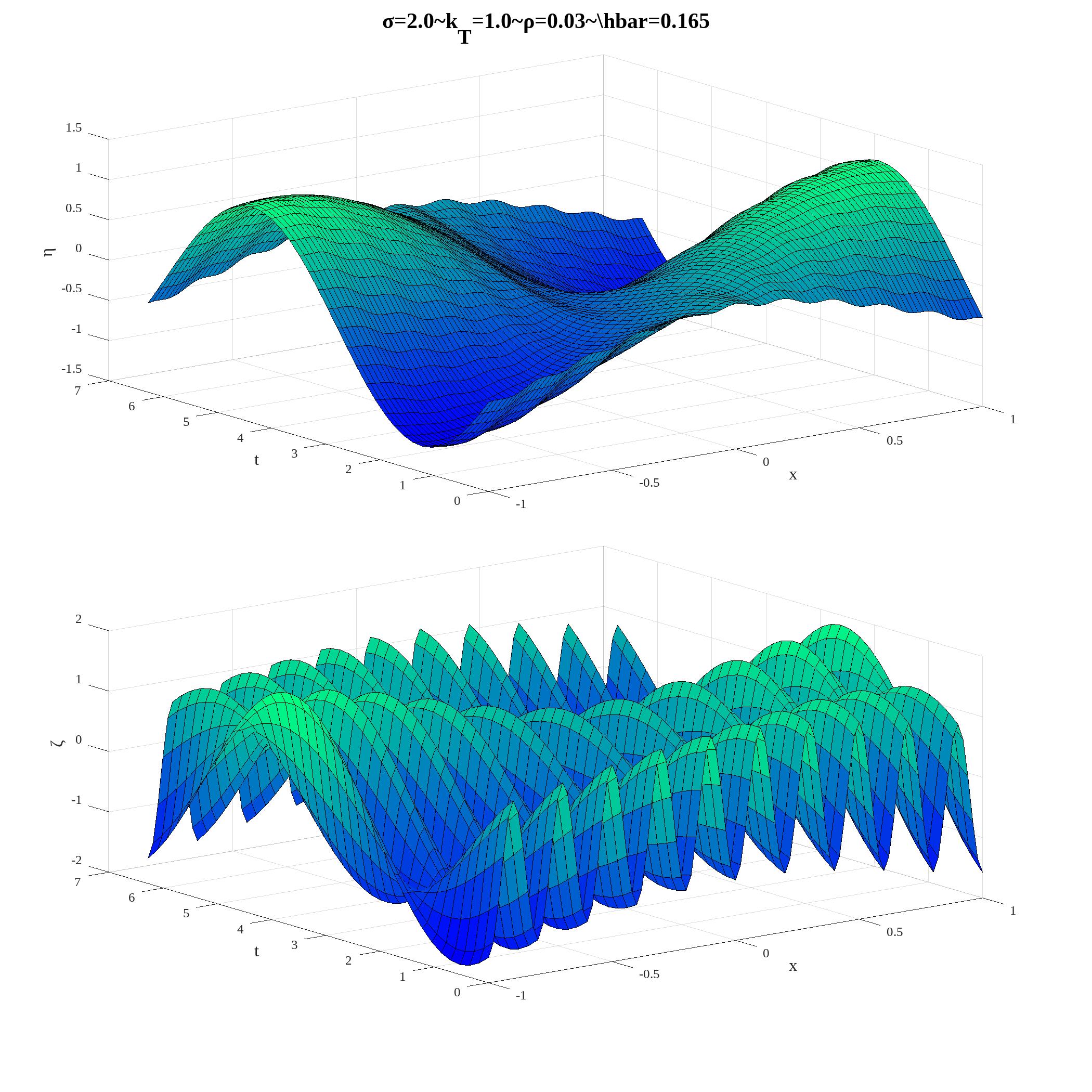
Figure 2.2: Analytic solution 2.24 for $\eta$ and $\zeta$ as functions of $x$ and $t$ .The parameter values are: $\kappa=2$ , $k=1$ ;, $\rho=0.03$ , $\hbar=0.165$

The solution for the surface, $\eta$ , and the interface, $\zeta$ , displacements are illustrated in figure 2.2. The sea level behaves consistently with the single layer solution (figure 1.2), exceptd for a high wavenumber modulation that is the surface signature of the interfacial motion. Conversely, the high wavenumber oscillation of the interface carry the signature of the surface displacement. The two modes are coupled.

2.2 FEM solution

2.2.1 System of 2 Second Order Equations

Weak Form

The weak form of the system 2.7 is:

	$\displaystyle\hbar\int\!\phi_{m}\frac{d^{2}N^{\prime}}{dx^{2}}\,dx$	$\displaystyle+$	$\displaystyle\kappa^{2}\int\!\phi_{m}(N^{\prime}-I)\,dx=-\kappa^{2}\int\!\phi_% {m}\overline{N}\,dx,$		(2.25)
	$\displaystyle\int\!\frac{d}{dx}\phi_{m}\left[(h-\hbar)\frac{d(N^{\prime}+\rho% \,I)}{dx}\right]\,dx$	$\displaystyle+$	$\displaystyle\kappa^{2}\int\!\phi_{m}I\,dx=0.$

If it is assumed that the depth varies little over an element, this becomes:

	$\displaystyle\hbar\int\!\phi_{m}\frac{d^{2}N^{\prime}}{dx^{2}}\,dx$	$\displaystyle+$	$\displaystyle\kappa^{2}\int\!\phi_{m}(N^{\prime}-I)\,dx=-\kappa^{2}\int\!\phi_% {m}\overline{N}\,dx,$		(2.26)
	$\displaystyle(h-\hbar)\int\!\phi_{m}\frac{d}{dx}\left[\frac{d(N^{\prime}+\rho% \,I)}{dx}\right]\,dx$	$\displaystyle+$	$\displaystyle\kappa^{2}\int\!\phi_{m}I\,dx=0.$

Following chapter 1, the integrals that involve second derivatives can be integrated by parts. Combining the result with the divergence theorem gives:

	$\displaystyle\hbar\int\!\frac{d\phi_{m}}{dx}\frac{d\,N^{\prime}}{dx}\,dx-% \kappa^{2}\int\!\phi_{m}(N^{\prime}-I)\,dx-\kappa^{2}\int\!\phi_{m}\overline{N% }\,dx$	$\displaystyle=$	$\displaystyle\left[\phi_{m}\frac{d\,N^{\prime}}{dx}\right]_{-1}^{1},$		(2.27)
	$\displaystyle(h-\hbar)\int\!\frac{d\phi_{m}}{dx}\frac{d(N^{\prime}+\rho\,I)}{% dx}\,dx-\kappa^{2}\int\!\phi_{m}I\,dx$	$\displaystyle=$	$\displaystyle(h-\hbar)\left[\phi_{m}\frac{d\,(N^{\prime}+\rho\,I)}{dx}\right]_% {-1}^{1}.$

The boundary condition 2.8 forces the terms on the right side of equation 2.27 to zero, so the sytem can be written:

	$\displaystyle\hbar\int\!\frac{d\phi_{m}}{dx}\frac{d\,N^{\prime}}{dx}\,dx-% \kappa^{2}\int\!\phi_{m}\,N^{\prime}\,dx+\kappa^{2}\int\!\phi_{m}\,I\,dx$	$\displaystyle=$	$\displaystyle\kappa^{2}\int\!\phi_{m}\overline{N}\,dx,$		(2.28)
	$\displaystyle(h-\hbar)\int\!\frac{d\phi_{m}}{dx}\frac{d(N^{\prime}+\rho\,I)}{% dx}\,dx-\kappa^{2}\int\!\phi_{m}I\,dx$	$\displaystyle=$	$\displaystyle 0.$

Assembly

Following equation 1.17, both dependent variables $N^{\prime}$ and $I$ are expanded in terms of the trial functions $\phi_{m}$ :

N^{\prime}(x)=\sum_{n=1}^{nx}\!N^{\prime}_{n}\phi_{n}(x)\quad I(x)=\sum_{n=1}^% {nx}\!I_{n}\phi_{n}(x),\quad\mbox{where}\quad\phi_{n}(x)=\sum_{m=1}^{M}\!C_{m,% n}x^{m-1}.

(2.29)

where $N^{\prime}_{n}$ and $I_{n}$ represent the solution at each node, and $n x$ is the total number of grid points.

With $\mathcal{M}$ (equation 1.21) and $\mathcal{K}$ the system 2.28 is:

\begin{bmatrix}\hbar\mathcal{K}-\kappa^{2}\mathcal{M}&\kappa^{2}\mathcal{M}\\ (h-\hbar)\mathcal{K}&-\kappa^{2}\mathcal{M}+\rho(h-\hbar)\mathcal{K}\end{% bmatrix}\bm{s}=\begin{bmatrix}\bm{F}\\ 0\end{bmatrix}\quad\mbox{where}\quad\bm{s}=\begin{bmatrix}N^{\prime}\\ I\end{bmatrix}

(2.30)

is the solution vector $\bm{s}$ consists of $n x$ values of $N^{\prime}$ followed by $n x$ values of $I$ . The matrix on the left of equation 2.30 is $2\,nx$ on side. Just as only the first of equations 2.7 is forced, there is only a load associated with the first set of equations. The load elements are given by

F_{m}=\kappa^{2}\int_{-1}^{1}\!\mathrm{e}^{-\mathrm{i}kx}\phi_{m}\,dx

(2.31)

Note the similarity between equation 1.22 and the system 2.30. In each case, $\bm{F}$ , $\bm{N^{\prime}}$ and $\bm{I}$ are complex.

Experience shows that when this problem is soleved as a system of two equations in two unknowns, quadratic TF are sufficient high polynomials to obtain an accurate solution. Once the global matrices and the load vector have been assembled, the solution is obtained by solving the usual linear system. The FEM solution is compared with the analytic solution 2.24 in figure 2.3.

Solutions to the forced two layer wave problem. The black
line represents the analytic solution, the blue line represents the
FEM solution with quadratic TF and the red line is the FEM
solution with cubic TF (described in the following section). The
cubic TF solution is a better match with the analytical solution. — Figure 2.3: Solutions to the forced two layer wave problem. The black line represents the analytic solution, the blue line represents the FEM solution with quadratic TF and the red line is the FEM solution with cubic TF (described in the following section). The cubic TF solution is a better match with the analytical solution.

Figure 2.3 is drawn with script C2S2figure3.m.

2.2.2 Single Fourth Order Equation

Weak Form

The starting point is equation 2.11 subject to conditions 2.12. With the exception of the fourth order derivative, each term has been considere in chapter 1. For a constant depth basin, with $\alpha=\rho\hbar(1-\hbar)$ , the extra term can be dealt with as follows:

\alpha\int\!\phi_{m}\frac{d^{4}N^{\prime}}{dx}\,dx=\alpha\int\!\frac{d}{dx}% \left(\phi\frac{d^{3}\,N^{\prime}}{dx^{3}}\right)\,dx-\alpha\int\!\frac{d\phi}% {dx}\frac{d^{3}\,N^{\prime}}{dx^{3}}\,dx=-\alpha\int\!\frac{d\phi}{dx}\frac{d^% {3}\,N^{\prime}}{dx^{3}}\,dx+\left(\phi\frac{d\,N^{\prime}}{dx}\right)_{-1}^{1}

(2.32)

after an integration by parts followed by application of the Divergence theorem (see section 1.2.1). The Divergence theorem can be used since $\phi$ is continuous. The second term on the right is zero because of the boundary condition. This process can be repeated a second time:

\alpha\int\!\phi_{m}\frac{d^{4}N^{\prime}}{dx}\,dx=-\alpha\int\!\frac{d}{dx}% \left(\frac{d\phi}{dr}\frac{d^{2}\,N^{\prime}}{dr}\right)\,dx+\alpha\int\!% \frac{d^{2}\phi}{dx^{2}}\frac{d^{2}\,N^{\prime}}{dx^{2}}\,dx

(2.33)

In order to use the Divergence theorem, the derivative of $\phi$ needs to be continuous, so test functions other that the linear and quadratic polynomials described in chapter 1 are required. These will be one-dimensional Hermite cubics, described in the following section. With the dependent variable $N^{\prime}$ expressed as an expansion over these functions, the weak form of equation 2.11 is:

\sum_{n}\left(\alpha\int_{-1}^{1}\!\frac{d^{2}\phi_{m}}{dx^{2}}\frac{d^{2}\phi% _{n}}{dx^{2}}\,dx-\beta\int_{-1}^{1}\!\frac{d\,\phi_{m}}{dx}\frac{d\,\phi_{n}}% {dx}\,dx+\kappa^{4}\int_{-1}^{1}\!\phi_{m}\phi_{n}\,dx\right)N^{\prime}_{n}=% \int_{-1}^{1}F\phi_{m}\,dx-\frac{\mathrm{i}\alpha\kappa^{2}\,k}{\hbar}\left(% \delta_{nx,m}\mathrm{e}^{-\mathrm{i}k}-\delta_{1,m}\mathrm{e}^{\mathrm{i}k}\right)

(2.34)

where $\beta=\kappa^{2}\left[1+\rho\,(1-\hbar)\right]$ . The last term on the right side of equation 2.34 represents the contribution from the boundary condition on $d^{3}N^{\prime}/dx^{3}$ . See lines 54 and 55 of NI2by2vs4.m

Cubic Test Functions

The test functions encountered in chapter 1 have all been continuous functions, but their derivatives (figure 1.4) are discontinuous. With hermite polynomial two (or more) functions test functions are defined at each node. In the case of Hermite cubic functions these are defined as:

\phi^{H}=(|x|-1)^{2}(2|x|+1),\quad\phi^{S}=x(|x|-1)^{2}

(2.35)

These are illustrated in figure 2.4. One function $\phi^{H}_{k}$ represent the height of the test function (equal to one at $x_{k}$ ) and the other accounts for the slope, and has a slope equal to one at $x_{k}$ .

Figure 2.4: The functions $\phi^{H}_{k}$ and $\phi^{S}_{k}$ . The amplitude of $\phi^{H}_{k}$ and the slope of $\phi^{S}_{k}$ is one at $x_{k}$

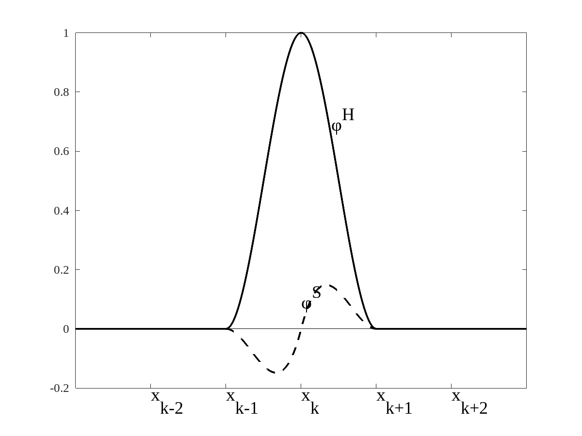
In this way both the function and its derivative are continuous. If there are $n x$ nodes, then there are $2\,nx$ test functions, and the global matrices are $2\,nx$ on side.

Assembly

For these cubic elements, the element mass matrix is:

\mathcal{M}e=\frac{\delta x}{420}\left(\begin{array}[]{c c c c}156&22\,\delta x% &54&-13\,\delta x\\ 22\,\delta x&4\,(\delta x)^{2}&13\,\delta x&-3(\delta x)^{2}\\ 54&13\,\delta x&156&-22\,\delta x\\ -13\,\delta x&-3(\delta x)^{2}&-22\,\delta x&4\,(\delta x)^{2}\end{array}\right)

(2.36)

The stiffness is

\mathcal{K}e=\frac{1}{30\delta x}\left(\begin{array}[]{c c c c}36&3\,\delta x&% -36&3\,\delta x\\ 3\,\delta x&4\,(\delta x)^{2}&-3\,\delta x&-(\delta x)^{2}\\ -36&-3\,\delta x&36&-3\,\delta x\\ 3\,\delta x&-(\delta x)^{2}&-3\,\delta x&4\,(\delta x)^{2}\end{array}\right)

(2.37)

and the fourth order stiffness matrix, defined as

\mathcal{K}^{iv}=\int_{-1}^{1}\!\frac{d^{2}\phi_{m}}{dx^{2}}\frac{d^{2}\phi_{n% }}{dx^{2}}\,dx

(2.38)

The elements of $\mathcal{K}e^{iv}$ are:

Ke^{iv}_{mn}=\frac{2}{(\delta x)^{3}}\begin{bmatrix}6&3\delta x&-6&3\delta x\\ 3\delta x&2(\delta x)^{2}&-3\delta x&(\delta x)^{2}\\ -6&-3\delta x&6&-3\delta x\\ 3\delta x&(\delta x)^{2}&-3\delta x&2(\delta x)^{2}\\ \end{bmatrix}

(2.39)

Assembly proceeds as in the previous chapter, on an element by element basis. The matrix equation to be solved for a single fourth order equation is:

\left(\alpha\mathcal{K}^{iv}-\beta\mathcal{K}+\kappa^{4}\mathcal{M}\right)\bm{% s}^{iv}=\bm{F}^{iv}

(2.40)

wher the solution vector is made up of pairs $N^{\prime H},N^{\prime S}$ at each node. The load vector is evaluated following equation 2.31, with additional contributions for the first and last nodes, corresponding to the last term on the right side of equation 2.34:

\bm{F}^{iv}=\kappa^{2}\begin{bmatrix}\int_{-1}^{1}F\phi_{1}\,dx+\frac{\mathrm{% i}\alpha\kappa^{2}\,k}{\hbar}\mathrm{e}^{\mathrm{i}k}\\ \vdots\\ \int_{-1}^{1}F\phi_{m}\,dx\\ \vdots\\ \int_{-1}^{1}F\phi_{2\,nx}\,dx-\frac{\mathrm{i}\alpha\kappa^{2}\,k}{\hbar}% \mathrm{e}^{-\mathrm{i}k}\end{bmatrix}

(2.41)

The Solution

Solutions to the forced two layer wave problem. The black
line represents the analytic solution, the green line represents
the FEM solution to a — Figure 2.5: Solutions to the forced two layer wave problem. The black line represents the analytic solution, the green line represents the FEM solution to a $2\times 2$ system with cubic TF and the blue line is the FEM solution to a $1\times 4$ system with cubic TF. For this case $nx=1001$ ,

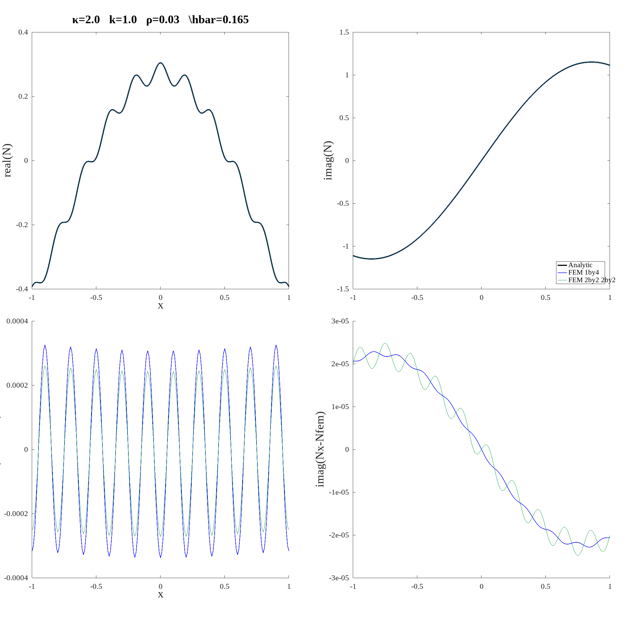
FEM solutions obtained with the system of two second order equations and with the single fourth order equation are compared with the analytic solution if figure 2.5. The upper two panels show the real and imaginar parts of the three solutions. Because they are nearly indistiguishable, the lower two panels illustrates differences between the analytic solution and the system of two second order equations solution (in green) and the single fourth order equation solution (blue line). These results suggest the system of two second order equations is preferable.

Exercises

1.

Write a script to reproduce figure 2.2 based on a FEM solution. Avoid looking at my scripts in this chapter.
2.

Modify script 2 to compute the forcing by quadrature. Under what conditions is this useful?

Scripts

Octave: Periodic Two Layer System: Quadratic vs Cubic Test Functions

⬇

%%ID C2S2: Two layer resposnse to equilibrium forcing

%%ID compare quadratic and cubic TF solutions to system of 2x2 equations

clear;

%% Problem parameters

rho=0.03;kappa=2;hbar=0.165;k=1;

nx=201;x=linspace(-1,1,nx);x=transpose(x);

%% Quad TF

tq=[(1:2:nx-2)’,(3:2:nx)’];ne=size(tq,1);dx=diff(x(1:2:3));

M=K=sparse(nx,nx);F=zeros(nx,1);

Me=dx*[4,2,-1;2,16,2;,-1,2,4]/30;

Ke=[7,-8,1;-8,16,-8;1,-8,7]/3/dx;

Fe=dx/6*[1;4;1];

%% F and K by quadrature

QuadWeights = [5/18,4/9,5/18];

QuadPoints = [0.5*(1-sqrt(0.6)),0.5,0.5*(1+sqrt(0.6))];

%% FEM Quadratic TF

for ke=1:ne

nodes=tq(ke,1):tq(ke,2);

M(nodes,nodes)=M(nodes,nodes)+Me;

K(nodes,nodes)=K(nodes,nodes)+Ke;

F(nodes,1)=F(nodes,1)+kappa^2*Fe*exp(-i*k*mean(x(nodes)));

endfor

L=[hbar*K-kappa^2*M,kappa^2*M;(1-hbar)*K,rho*(1-hbar)*K-kappa^2*M];

s = L\[F;zeros(nx,1)];

Nquad = s (1:nx)+exp(-i*k*x);

Iquad = s (nx+1:2*nx);

%%% FEM cubic trial fn

tc=[(1:nx-1)’,(2:nx)’];dx=diff(x(1:2));␣%same␣dx␣as␣linear␣TF␣half␣of␣quad␣TF

M=K=sparse(2*nx,2*nx);F=zeros(2*nx,1);

Ke=[36,3*dx,-36,3*dx;␣…

␣␣␣␣3*dx,4*dx^2,-3*dx,-dx^2;␣…

␣␣␣␣-36,-3*dx,36,-3*dx;␣…

␣␣␣␣3*dx,-dx^2,-3*dx,4*dx^2]/30/dx;

Me=dx*[156,22*dx,54,-13*dx;␣…

␣␣␣␣␣␣␣22*dx,4*dx^2,13*dx,-3*dx^2;␣…

␣␣␣␣␣␣␣54,13*dx,156,-22*dx;␣…

␣␣␣␣␣␣␣-13*dx,-3*dx^2,-22*dx,4*dx^2]/420;

for␣e=1:nx-1

␣␣nodes=tc(e,:);ind=2*(tc(e,1)-1)+[1:4];

␣␣Fe(1:2,1)=kappa^2*dx/12*[6;dx]*exp(-i*k*x(nodes(1)));

␣␣Fe(3:4,1)=kappa^2*dx/12*[6;-dx]*exp(-i*k*x(nodes(2)));

␣␣K(ind,ind)=K(ind,ind)+Ke;

␣␣M(ind,ind)=M(ind,ind)+Me;

␣␣F(ind,1)=F(ind,1)+Fe;

end

L=[hbar*K-kappa^2*M,kappa^2*M;(1-hbar)*K,rho*(1-hbar)*K-kappa^2*M];

s␣=␣L\[F;zeros(2*nx,1)];

Ncub␣=␣s␣(1:2:2*nx)+exp(-i*k*x);

Icub␣=␣s␣(2*nx+1:2:4*nx);

%%␣Exact␣solution

[N,I]=NIexacthcons(nx,kappa,k,rho,hbar);N=transpose(N);I=transpose(I);

%%␣Plots

set(gcf,”position”,[500,10,1400,1400]);clf

axes(’position’,[0.05,0.55,0.4,0.4]);plot(x,real(N),’k’,’linewidth’,2);

hold␣on;plot(x,real(Nquad),’b’,’linewidth’,1);%axis([-1,1,-.4,.4]);

plot(x,real(Ncub),’color’,[0,0.6,0.2],’linewidth’,1/2);

xlabel(’x’,’fontsize’,18);ylabel(’real(N)’,’fontsize’,18);

title(strcat(’\kappa=’,num2str(kappa,’%3.1f’),{’␣␣␣k=’},num2str(k,’%3.1f’),{’␣␣␣\rho=’},num2str(rho,’%3.2f’),{’␣␣␣\hbar=’},num2str(hbar,’%4.3f’)),’fontsize’,18);

axes(’position’,[0.55,0.55,0.4,0.4]);plot(x,imag(N),’k’,’linewidth’,2);

hold␣on;plot(x,imag(Nquad),’b’,’linewidth’,1);

plot(x,imag(Ncub),’color’,[0,0.6,0.2],’linewidth’,1/2);ylabel(’imag(N)’,’fontsize’,18);

legend(’Analytic’,’FEM␣2by2␣quad’,’FEM␣2by2␣cub’,’location’,’southeast’)

axes(’position’,[0.05,0.1,0.4,0.4]);plot(x,real(I),’k’,’linewidth’,2);

hold␣on;plot(x,real(Iquad),’b’,’linewidth’,1);axis([-1,1,-.4,.4]);

plot(x,real(Icub),’color’,[0,0.6,0.2],’linewidth’,1/2);axis([-1,1,-2,2]);

xlabel(’x’,’fontsize’,18);ylabel(’real(I)’,’fontsize’,18);

axes(’position’,[0.55,0.1,0.4,0.4]);plot(x,imag(I),’k’,’linewidth’,2);

hold␣on;plot(x,imag(Iquad),’b’,’linewidth’,1);

plot(x,imag(Icub),’color’,[0,0.6,0.2],’linewidth’,1/2);ylabel(’imag(I)’,’fontsize’,18);

set(gcf,’paperpositionmode’,’manual’,’paperposition’,[0.25␣0.25␣14␣14])

print␣-dpng␣../../words/figs/C2/C2S2figure3.png

Octave: Periodic Two Layer System: Fourth Order vs System of Second Order

⬇

%%ID C2S2: Two layer resposnse to equilibrium forcing

%%ID compare cubic TF solutions in a 2by2 vs 1by4 formulation

clear

%% Problem parameters

rho=0.03;kappa=2;hbar=0.165;k=1;

%% F(orcing)

nx=201;x=linspace(-1,1,nx);x=transpose(x);dx=diff(x(1:2));

%% FEM 2x2 cubic trial fn

tc=[(1:nx-1)’,(2:nx)’];dx=diff(x(1:2));␣%same␣dx␣as␣linear␣TF␣half␣of␣quad␣TF

M=K=sparse(2*nx,2*nx);F=zeros(2*nx,1);

Ke=[36,3*dx,-36,3*dx;␣…

␣␣␣␣3*dx,4*dx^2,-3*dx,-dx^2;␣…

␣␣␣␣-36,-3*dx,36,-3*dx;␣…

␣␣␣␣3*dx,-dx^2,-3*dx,4*dx^2]/30/dx;

Me=dx*[156,22*dx,54,-13*dx;␣…

␣␣␣␣␣␣␣22*dx,4*dx^2,13*dx,-3*dx^2;␣…

␣␣␣␣␣␣␣54,13*dx,156,-22*dx;␣…

␣␣␣␣␣␣␣-13*dx,-3*dx^2,-22*dx,4*dx^2]/420;

for␣e=1:nx-1

␣␣nodes=tc(e,:);ind=2*(tc(e,1)-1)+[1:4];

␣␣Fe(1:2,1)=kappa^2*dx/12*[6;dx]*exp(-i*k*x(nodes(1)));

␣␣Fe(3:4,1)=kappa^2*dx/12*[6;-dx]*exp(-i*k*x(nodes(2)));

␣␣K(ind,ind)=K(ind,ind)+Ke;

␣␣M(ind,ind)=M(ind,ind)+Me;

␣␣F(ind,1)=F(ind,1)+Fe;

end

L=[hbar*K-kappa^2*M,kappa^2*M;(1-hbar)*K,rho*(1-hbar)*K-kappa^2*M];

s␣=␣L\[F;zeros(2*nx,1)];

N2by2␣=␣s␣(1:2:2*nx)+exp(-i*k*x);

I2by2␣=␣s␣(2*nx+1:2:4*nx);%␣not␣used␣here

%%␣␣FEM␣1x4␣cubic␣trial␣fn

alpha=rho*hbar*(1-hbar);beta=kappa^2*(1+rho*(1-hbar));

gamma=g=kappa^2*(rho*(1-hbar)*k^2-kappa^2);

K4=sparse(2*nx,2*nx);F=zeros(2*nx,1);

K4e=2*[6,3*dx,-6,3*dx;␣…

␣␣␣␣␣␣␣3*dx,2*dx^2,-3*dx,dx^2;␣…

␣␣␣␣␣␣␣-6,-3*dx,6,-3*dx;␣…

␣␣␣␣␣␣␣3*dx,dx^2,-3*dx,2*dx^2]/dx^3;

%%␣M␣and␣K␣are␣identical␣to␣values␣given␣above

for␣e=1:nx-1

␣␣nodes=tc(e,:);ind=2*(tc(e,1)-1)+[1:4];

␣␣K4(ind,ind)=K4(ind,ind)+K4e;

␣␣Fe(1:2,1)=gamma*dx/12*[6;dx]*exp(-i*k*x(nodes(1)));

␣␣Fe(3:4,1)=gamma*dx/12*[6;-dx]*exp(-i*k*x(nodes(2)));

␣␣F(ind)=F(ind)+Fe;

end

%%␣Adjust␣rhs␣(F^iv)␣for␣bc␣on␣d^3N’/dx^3

F(1,1)=F(1,1)+i*alpha*kappa^2*k*exp(i*k)/hbar;

F(2*nx-1,1)=F(2*nx-1,1)-i*alpha*kappa^2*k*exp(-i*k)/hbar;

%%␣because␣the␣BC␣on␣dN’/dx␣is␣homogeneous,␣we␣only␣include

%%␣equations␣for␣N’^H␣at␣extremities␣(-1<=x<=1)

K4=[K4(1,1),K4(1,3:2*nx-1);K4(3:2*nx-1,1),K4(3:2*nx-1,3:2*nx-1)];

K=[K(1,1),K(1,3:2*nx-1);K(3:2*nx-1,1),K(3:2*nx-1,3:2*nx-1)];

M=[M(1,1),M(1,3:2*nx-1);M(3:2*nx-1,1),M(3:2*nx-1,3:2*nx-1)];

F=[F(1,1);F(3:2*nx-1,1)];

%%␣Solve␣linear␣system

s=(alpha*K4-beta*K+kappa^4*M)\F;

%%␣sort␣out␣s␣into␣N’^H␣and␣N’^S␣(unused␣here)

NpH=[s(1);s(2:2:2*(nx-1))];NpS=[s(2:2*nx-2)];

N1by4=NpH+exp(-i*k*x);␣%␣add␣Nbar␣tp␣Nprime␣to␣get␣N

%%␣if␣I␣was␣needed␣get␣it␣from␣equation␣2.9

%%␣get␣exact␣solution

[Nx,Ix]=NIexacthcons(nx,kappa,k,rho,hbar);Nx=transpose(Nx);Ix=transpose(Ix);

set(gcf,”position”,[100,1000,1400,1400]);clf

axes(’position’,[0.05,0.55,0.4,0.4]);plot(x,real(Nx),’k’,’linewidth’,2);

hold␣on;plot(x,real(N1by4),’b’,’linewidth’,1);axis([-1,1,-.4,.4]);

plot(x,real(N2by2),’color’,[0,0.6,0.2],’linewidth’,1/2);axis([-1,1,-.4,.4]);

xlabel(’x’,’fontsize’,18);ylabel(’real(N)’,’fontsize’,18);

axes(’position’,[0.55,0.55,0.4,0.4]);plot(x,imag(Nx),’k’,’linewidth’,2);

hold␣on;plot(x,imag(N1by4),’b’,’linewidth’,1);

plot(x,imag(N2by2),’color’,[0,0.6,0.2],’linewidth’,1/2);ylabel(’imag(N)’,’fontsize’,18);

legend(’Analytic’,’FEM␣1by4’,’FEM␣2by2␣2by2’,’location’,’southeast’)

axes(’position’,[0.05,0.1,0.4,0.4]);

hold␣on;plot(x,real(Nx-N1by4),’b’,’linewidth’,1);

plot(x,real(Nx-N2by2),’color’,[0,0.6,0.2],’linewidth’,1/2);

xlabel(’x’,’fontsize’,18);ylabel(’real(Nx-Nfem)’,’fontsize’,18);

axes(’position’,[0.55,0.1,0.4,0.4]);

hold␣on;plot(x,imag(Nx-N1by4),’b’,’linewidth’,1);

plot(x,imag(Nx-N2by2),’color’,[0,0.6,0.2],’linewidth’,1/2);ylabel(’imag(Nx-Nfem)’,’fontsize’,18);

set(gcf,’paperpositionmode’,’manual’,’paperposition’,[0.25␣0.25␣14␣14])

print␣-dpng␣../../words/figs/C2/C2S2figure5.png