Notes on the Finite Element Method 2 Tides in a Two-layer Fluid: Solving a System of Equations 4 Two Dimensional Potential Flows

Chapter 3 Time-dependent Waves and Burgers’ Equation

In many cases of practical importance, the system of interest evolves in time in such a way that the assumption of periodic motion is not useful. Describing the temporal evolution requires integrating the governing equations forward in time. Two examples involving problem that are one-dimensional in space are treated: the time dependent linear wave equation and the non-linear Burgers equation.

3.1 The Wave Equation Revisited

When selecting a method well-suited to step a solution forward in time, two questions arise: is the method stable and if it is how accurate is it. These issues are discussed in the next section.

3.1.1 Stability and Accuracy

Discretizing a differential equation can introduce spurious solutions. If these extraneous solutions grow, the computed solution will bear no resemblance to the exact solution (for example it might grow exponentially in time). Stability analysis provides a means to determine whether the solution to the discretized problem remains close to the real solution. Accuracy deals with the magnitude of differences between a computed solution and the analytical solution.

As far as accuracy is concerned, a classical example discussed by Strang (pp117-119) concerns a spring-mass system where the position of the mass is $X(t)$ . The velocity of the mass is $u=dX/dt$ . The force balance governing $X$ is:

\frac{d^{2}X}{dt^{2}}+X=0

(3.1)

Write the problems as a system of two first order equations:

\frac{dX}{dt}=u,\quad u=-\frac{dX}{dt}

(3.2)

where $u$ is the velocity of the mass. At $t=0$ the mass is displaced to $X=1$ , and the velocity is zero. If the time dependence is discretized into chunks of length $\delta t$ , there are several ways to integrate system 3.2 forward in time. Strang compares the following four schemes:

Forward Euler

X^{t+\delta t}=X^{t}+\delta t\,U^{t},\quad U^{t+\delta t}=U^{t}-\delta t\,X^{t% }\quad\mbox{or}\quad\begin{bmatrix}X\\ U\end{bmatrix}^{t+\delta t}=\mathcal{G}_{F}\begin{bmatrix}X\\ U\end{bmatrix}^{t}\quad\mbox{where}\quad\mathcal{G}_{F}=\begin{bmatrix}1&% \delta t\\ -\delta t&1\end{bmatrix}

(3.3)

This scheme is explicit, meaning that the solution a the new time depends solely on quantities evaluated at an earlier time. For this reason it is known as the Forward Euler method. The matrix $\mathcal{G}$ is the growth matrix. The growth factor is $|\mathcal{G}|$ , the determinant of $\mathcal{G}$ . In this case $|\mathcal{G}_{f}|=1+(\delta t)^{2}$ . The method is conditionally stable and errors grow.

Backward Euler

X^{t+1}=X^{t}+\delta t\,U^{t+1},\quad U^{t+1}=U^{t}-\delta t\,X^{t+1},\quad% \mbox{or}\quad\begin{bmatrix}X\\ U\end{bmatrix}^{t+\delta t}=\begin{bmatrix}1&-\delta t\\ \delta t&1\end{bmatrix}^{-1}\begin{bmatrix}X\\ U\end{bmatrix}^{t}.

(3.4)

The Backward Euler methoid is implicit. The growth factor is $|\mathcal{G}_{f}|=(1+(\delta t)^{2})^{-1}$ , always less than one. The method is stabl Terms evaluated at the new time step $t+1$ appear on the right hand side.

Trapezoidal Method

The Trapezoidal method is also implicit:

X^{t+1}=X^{t}+\delta t(U^{t+1}+U^{t})/2,\quad U^{t+1}=U^{t}-\delta t(X^{+1}+X^% {t})/2\;\mbox{or}\;\begin{bmatrix}X\\ U\end{bmatrix}^{t+\delta t}\!=\frac{1}{4}\begin{bmatrix}2&-\delta t\\ \delta t&2\end{bmatrix}^{-1}\begin{bmatrix}2&\delta t\\ -\delta t&2\end{bmatrix}\begin{bmatrix}X\\ U\end{bmatrix}^{t}.

(3.5)

Now the growth factor is $|\mathcal{G}_{t}|=1$ . This is a second-order method, is the method of choice for integrating time-dependent problems (with the exception of stiff problems).

Leapfrog Method

The only drawback to the Trapezoidal method is that it is implicit, requiring a matrix inversion at each time step. The Leapfrog method is:

X^{t+1}=X^{t}+\delta t\,U^{t},\quad U^{t+1}=U^{t}-\delta t\,X^{t+1},\quad\mbox% {or}\quad\begin{bmatrix}X\\ U\end{bmatrix}^{t+\delta t}=\begin{bmatrix}1&\delta t\\ -\delta t&1-(\delta t)^{2}\end{bmatrix}^{-1}\begin{bmatrix}X\\ U\end{bmatrix}^{t}.

(3.6)

The growth factor is also $|\mathcal{G}_{l}|=1$ .

Each scheme has been used to integrate system 3.2 forward from $t=0$ to $t=2\pi$ , and the results are compared in figure 3.1, where the dependent variable $u$ is show as a function of the other dependent variable $X$ .

Figure 3.1: Phase diagram showing velocity $u$ as a function of position $X$ for four different integrations schemes. (see Strang, pg 117-118). The dashed circle represents the exact solution. In all cases, $\delta t=1\pi/36$ ; the symbol represents the solution in $X-u$ space, with the solid symbol marking the initial position. Redrawn from Strang

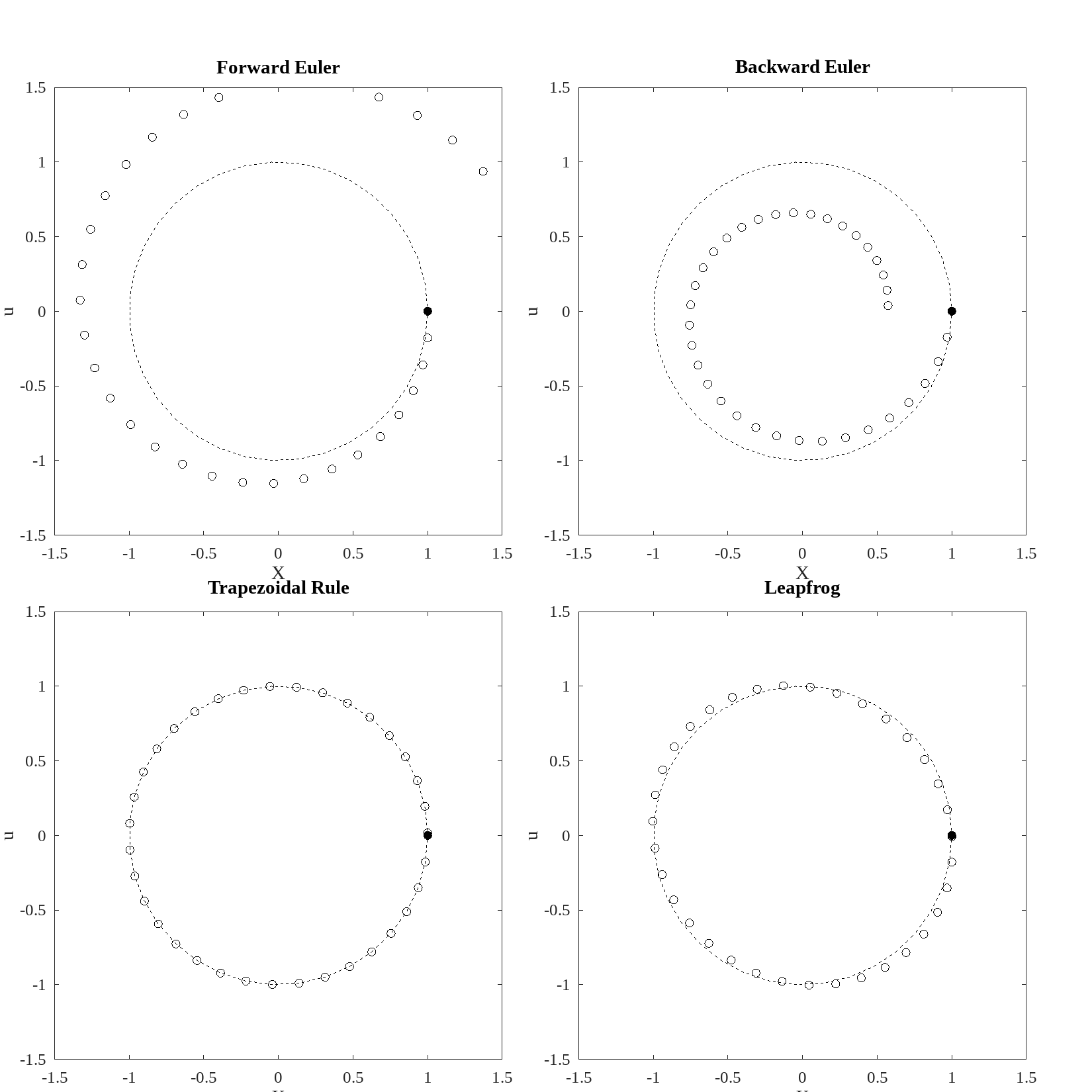
The two Euler solutions rapidly diverge from the exact solution (the black circle): the accuracy is low. The trapezoidal solution, stay on the circle, however there is a small phase error at the end of a cycle. The leapfrog method has no phase error, but the amplitudes varies by a small amount so that the numerical solution traces an ellipse in the phase plane. The last two methods are much more accurate than the two Euler methods.

3.1.2 The Wave Equation

The wave equation is a good test bed to evaluate the stabilty of the four numerical schemes described above. Consider the system

\frac{\partial\eta}{\partial t}+\frac{\partial(hu)}{\partial x}=0,\quad\frac{% \partial u}{\partial t}=-g\frac{\partial\eta}{\partial x}

(3.7)

Difference between the solution computed by each scheme and
the exact solution at time — Figure 3.2: Difference between the solution computed by each scheme and the exact solution at time $t=2$ . The Forward Euler scheme is unstable. The Trapezoidal scheme works well so long as $\delta t<\delta x$ . The error associated withleapfrog is larger than trapezoidal. For these calculations $\delta x=\delta t=4\cdot 10{-3}$ .

The weak form is:

\frac{\partial}{\partial t}\int_{-L}^{L}\!\phi_{m}\,\eta\,dx+\int_{-L}^{L}\!% \phi_{m}\,\frac{\partial(hu)}{\partial x}\,dx=0\quad\frac{\partial}{\partial t% }\int_{-L}^{L}\!\phi_{m}\,u\,dx+gh\int_{-L}^{L}\!\phi_{m}\,\frac{\partial\eta}% {\partial x}\,dx=0

(3.8)

Write the time index as a superscript; the solutions $u^{t}(x)$ and $\eta^{t}(x)$ are written as expansions in the trial functions:

u^{t}(x)=\sum_{n=1}^{nx}u^{t}_{n}\phi_{n}\quad\eta^{t}(x)=\sum_{n=1}^{nx}\eta^% {t}_{n}\phi_{n}

(3.9)

Introducing these expansions into equation 3.8

\sum_{n=1}^{nx}\frac{\partial\eta_{n}^{t}}{\partial t}\int_{-L}^{L}\!\phi_{m}% \,\phi_{n}\,dx+\sum_{n=1}^{nx}u_{n}\int_{-L}^{L}\!\phi_{m}\,\frac{\partial\phi% _{n}}{\partial x}\,dx=0

(3.10)

gh\sum_{n=1}^{nx}\int_{-L}^{L}\!\phi_{m}\,\frac{\partial\phi_{n}}{\partial x}% \,\eta_{n}^{t}\,dx+\sum_{n=1}^{nx}\frac{\partial u_{n}^{t}}{\partial t}\int_{-% L}^{L}\!\phi_{m}\,\phi_{n}\,dx=0

(3.11)

With the new FEM element matrix:

De_{mn}=\int\!\phi_{m}\frac{\partial\phi_{n}}{\partial x}\,dx

(3.12)

For linear TF, Maxima gives:

De_{mn}=\frac{1}{2}\begin{bmatrix}-1&1\\ -1&1\end{bmatrix}

(3.13)

Form the global matrices from the element matrices in the usual way. The system of equations becomes

\mathcal{M}\frac{\partial\bm{\eta}^{t}}{\partial t}+\mathcal{D}^{T}\bm{u}^{t}=% 0,\quad c^{2}\mathcal{D}\bm{\eta}^{t}+\mathcal{M}\frac{\partial\bm{u}^{t}}{% \partial t}=0

(3.14)

The Forward Euler scheme is achieved by stepping:

\begin{bmatrix}\mathcal{M}&0\\ 0&\mathcal{M}\end{bmatrix}\begin{bmatrix}\bm{\eta}^{t+1}\\ \bm{u}^{t+1}\end{bmatrix}=\begin{bmatrix}\mathcal{M}&-\delta t\mathcal{D}\\ -\delta t\mathcal{D}&\mathcal{M}\end{bmatrix}\begin{bmatrix}\bm{\eta}^{t}\\ \bm{u}^{t}\end{bmatrix}

(3.15)

forward. This is an explicit scheme.

For the Backward Euler scheme step:

\begin{bmatrix}\mathcal{M}&\delta t\mathcal{D}\\ \delta t\mathcal{D}&\mathcal{M}\end{bmatrix}\begin{bmatrix}\bm{\eta}^{t+1}\\ \bm{u}^{t+1}\end{bmatrix}=\begin{bmatrix}\mathcal{M}&0\\ 0&\mathcal{M}\end{bmatrix}\begin{bmatrix}\bm{\eta}^{t}\\ \bm{u}^{t}\end{bmatrix}

(3.16)

For the Trapezoidal scheme, step

\begin{bmatrix}\mathcal{M}&\delta t\mathcal{D}/2\\ \delta t\mathcal{D}/2&\mathcal{M}\end{bmatrix}\begin{bmatrix}\bm{\eta}^{t+1}\\ \bm{u}^{t+1}\end{bmatrix}=\begin{bmatrix}\mathcal{M}&-\delta t\mathcal{D}/2\\ -\delta t\mathcal{D}/2&\mathcal{M}\end{bmatrix}\begin{bmatrix}\bm{\eta}^{t}\\ \bm{u}^{t}\end{bmatrix}

(3.17)

and for the Leapfrog scheme

\begin{bmatrix}\mathcal{M}&\delta t\mathcal{D}\\ 0&\mathcal{M}\end{bmatrix}\begin{bmatrix}\bm{\eta}^{t+1}\\ \bm{u}^{t+1}\end{bmatrix}=\begin{bmatrix}\mathcal{M}&0\\ -\delta t\mathcal{D}&\mathcal{M}\end{bmatrix}\begin{bmatrix}\bm{\eta}^{t}\\ \bm{u}^{t}\end{bmatrix}

(3.18)

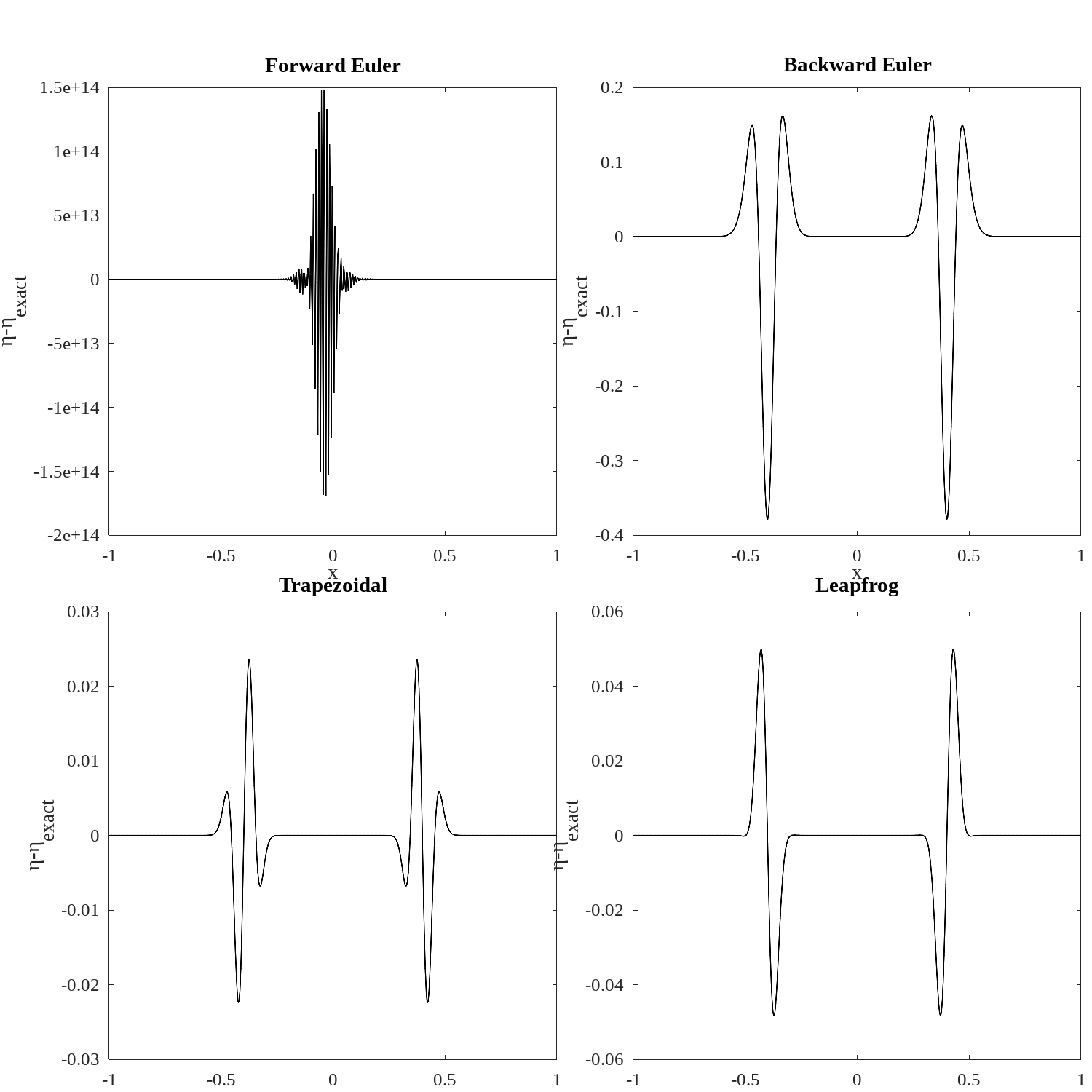
Consider a wave system where a gaussian bump of water is released from $x=0$ at $t=0$ . With d’Alemebert’s solution it is clear that two gaussian bumps, each half the height of the original disturbance, will propgaten away from the center, one toward $+x$ , and the other toward $-x$ . The solution obtained by integrating the equations with each scheme over a two second period is illustrated in figure 3.2, as difference between the computed and exact solution. The Forward Euler scheme goes unstable immediately, as would any other explicit scheme. The error associated with the Trapezoidal scheme is the smallest, and diminishes as the number of elements squared. The trapezoidal scheme is said to be L-stable. We will adopt this scheme for the rest of the class with one exception: for stiff problems, such as the incompressible Navier-Stokes equations, methods that are L-stable are required.

The two components of equation 3.7 can be combined into the wave equation:

c^{2}\frac{\partial^{2}\eta}{\partial x^{2}}+\frac{\partial^{2}\eta}{\partial x% ^{2}}=0

(3.19)

for simplicity the phase speed is assumed $c=1$ . If the boundary conditions guarantee that the variable satisfies homogeneous Neumann conditions (corresponding to zero mass flux through the boundaries),, the weak version in matrix form is

\frac{\partial^{2}}{\partial t^{2}}\left(\mathcal{M}\bm{\eta}\right)=-\mathcal% {K}\bm{\eta}

(3.20)

Now we replace the second derivatime in time by centered differences:

\mathcal{M}\left(\bm{\eta}^{t+1}-2\bm{\eta}^{t}+\bm{\eta}^{t-1}\right)=-(% \delta t)^{2}\mathcal{K}\bm{\eta}^{t}

(3.21)

Figure 3.3: Surface elevations, $\eta$ as a function of position $x$ and time $t$ . The initial bulge separates into two half height waves that propagate toward the basin extremities. The locus of the peaks follows the characteristics emananating from $x=0$ at $t=0$ . At $t=1$ they reflect back into the basin. Without friction the process would go on forever.

This scheme requires initial values at two times. Fortunately we have the d’Alembert solution, so for a Gaussian bump at $t=0$ , start with:

\eta(x,0)=2\mathrm{e}^{-\alpha x^{2}},\quad\eta(x,-\delta t)=\mathrm{e}^{-% \alpha(x-c\delta t)^{2}}+\mathrm{e}^{-\alpha(x+c\delta t)^{2}}

(3.22)

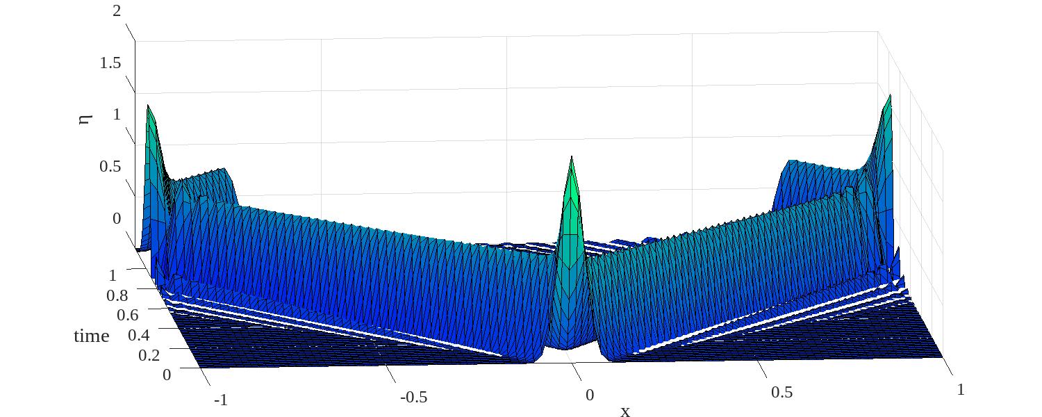
The solution $\eta(x,t)$ for a case where $c=1$ is illustrated in figure 3.3. As time increase the initial disturbance produces two faves, each progressing toward opposite ends of the basin, where they reflect and head back toward the center of the basin. The ridges of maximum $\eta$ trace out the characteristics emanating from $x=0$ at $t=0$ .

3.2 Burgers’ Equation

Read Strang pg 537

Burgers equation is:

\frac{\partial u}{\partial t}+u\frac{\partial u}{\partial x}=\nu\frac{\partial% ^{2}u}{\partial x^{2}}

(3.23)

In the following three different exact solutions to Burgers’ equation are reviewed.

3.2.1 Characteristics, Expansions and Shocks

If the viscosity $\nu=0$ , Burgers equation looks like the one-way wave equation. Do characteristics exist? Define $\xi=x-ut$ . Then, with the chain rule:

\frac{\partial}{\partial x}=\frac{d}{d\xi}\frac{\partial\xi}{\partial x}=\frac% {d}{d\xi},\quad\frac{\partial}{\partial t}=\frac{d}{d\xi}\frac{\partial\xi}{% \partial t}=-u\frac{d}{d\xi}.

(3.24)

Therefore any function $g(\xi)$ satisfies the inviscid Burgers equation.

-u\frac{d\,g}{d\xi}+u\frac{d\,g}{d\xi}\equiv 0.

(3.25)

The function $g$ is constant along characteristic lines. Hovever, in contrat to the linear case, the characteristics need no longer remain parallel, as illustrated by the solid black lines illustrated on the $u=0$ plane in figure 3.4. At $time=0$ the initial profile is a gaussian function of $x$ , symmetric relative to $x=0$ . As time increases the non-linearity distorts the initial profile in such a way that area where the velocity increases with $x$ expand and areas where the velocity decrease with $x$ sharpen. Eventually these area will contain shocks, where the Riemann solutions take over, as illustrated in figure 3.4.

Figure 3.4: Solution to Burgers equation with $\nu=0$ . Velocity $u$ as a function of position $x$ and time $t$ . Initially the velocity bulge is symmetric about $x=0$ . The characteristics, shown as black lines on the $x$ - $t$ plane, tend to coalesce in the region where the flow is deccelerating, and expand where the flow accelerates. As a result the velocity bulge evolves in shape, steepening in the region where the streamlines converge.

3.2.2 Solution for a Translating Front

Returning to the full Bergers equation, look for solutions of the form $u(\zeta)$ where $\zeta=x-ct$ , and the constant wave speed $c$ is to be determined. The initial condition is $u\rightarrow u_{1}$ as $x\rightarrow\infty$ and $u\rightarrow u_{2}$ as $x\rightarrow-\infty$ . If we introduce the new independent variable into equation 3.23 we get:

-c\frac{d\,u}{d\zeta}+u\frac{d\,u}{d\zeta}=\nu\frac{d^{2}u}{d\zeta^{2}}

(3.26)

Try a solution of the form

u=a+b\,\tanh{(\alpha\zeta)}

(3.27)

Equation 3.26 becomes

\frac{b\alpha(a-c)}{\cosh^{2}{(\alpha\,\xi)}}+\frac{b\alpha(b+2\alpha\nu)\tanh% {(\alpha\,\xi)}}{\cosh^{2}{(\alpha\,\xi)}}=0

(3.28)

The choices

a=c\quad\mbox{and}\quad b=-2\alpha\nu

(3.29)

turn equation 3.28 into an identity. The boundary conditions then determine $a$ and $b$ so the solution is

u=\overline{u}+\frac{\delta u}{2}\tanh{\frac{\delta u\,\zeta}{4\nu}}\quad\mbox% {where}\quad\zeta=x-\overline{u}\,t.

(3.30)

Figure 3.5: Velocity $u$ (equation 3.30) as a function of position $x$ for three values of the viscosity $\nu$ . For this calculation $\overline{u}=\delta u=1.$ .

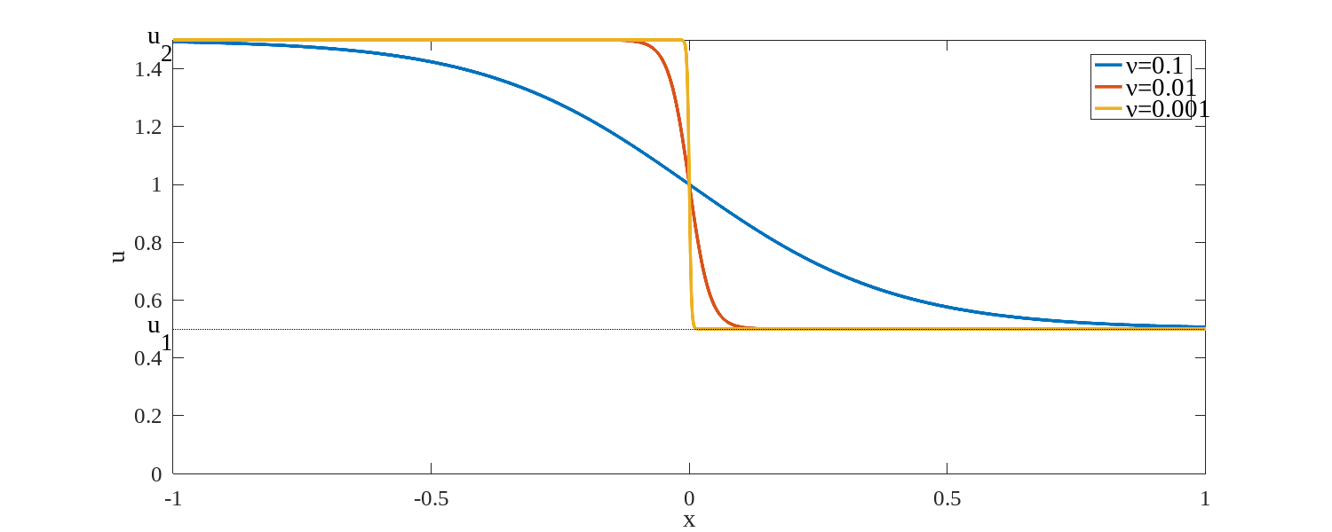
This solution is illustrated in figure 3.5 for several values of the ratio $\delta u/\nu$ . The form of the solution shows that the wavefront remains locally unchanges, moving to the right at the average speed of the two streams.

3.2.3 A second solution: the Cole-Hopf transformation

Consider equation 3.23 with initial and BC:

u(x,0)=\delta(x),\quad u(\pm\infty,t)=0.

(3.31)

Make the transformation $\psi_{x}=u$ and integrate once in x to get an equation for $\psi$ :

\frac{\partial\psi}{\partial t}+\frac{1}{2}\left(\frac{\partial\psi}{\partial x% }\right)^{2}=\nu\frac{\partial^{2}\psi}{\partial x^{2}}

(3.32)

make the further transformation $\psi=-4\ln{\phi}/\mbox{Re}$ , equivalent to:

u=-2\nu\frac{\phi_{x}}{\phi}

(3.33)

the derivatives are:

\frac{\partial\psi}{\partial t}=-\frac{2\nu}{\phi}\frac{\partial\phi}{\partial t% };\quad\frac{\partial\psi}{\partial x}=-\frac{2\nu}{\phi}\frac{\partial\phi}{% \partial x};\quad\frac{\partial^{2}\psi}{\partial x^{2}}=\frac{2\nu}{\phi^{2}}% \left[\left(\frac{\partial\phi}{\partial x}\right)^{2}-\phi\frac{\partial^{2}% \phi}{\partial x^{2}}\right]

(3.34)

substitute into equation 3.32:

-\frac{2\nu}{\phi}\frac{\partial\phi}{\partial t}+2\left(\frac{\nu}{\phi}\frac% {\partial\phi}{\partial x}\right)^{2}=2\left(\frac{\nu}{\phi^{2}}\right)^{2}% \left[\left(\frac{\partial\phi}{\partial x}\right)^{2}-\phi\frac{\partial^{2}% \phi}{\partial x^{2}}\right]

(3.35)

and the equation for $\phi$ is:

\frac{\partial\phi}{\partial t}=\nu\frac{\partial^{2}\phi}{\partial x^{2}}

(3.36)

This is the heat equation. The initial condition the the various dependent variables are:

u(x,0)=\delta(x),\quad\psi(x,0)=H(x),\quad\phi(x,0)=\exp{(-\frac{H(x)}{2\nu})}

(3.37)

Initially $\phi$ has a step change where $x=0$ . The problem for $\phi$ is identical to the linearized shear layer problem, and the solution is known to be of the form:

\phi=a+b\,\mathrm{erf}(\eta)\quad\mbox{where}\quad\eta=\sqrt{\frac{x^{2}}{4\nu% \,t}}

(3.38)

The constants $a$ and $b$ are determined by the boundary conditions:

\phi(-\infty)=1,\quad\phi(\infty)=\mathrm{e}^{-1/(2\nu)}

(3.39)

The function $\phi$ becomes:

\phi=\frac{1+\mathrm{e}^{-1/(2\nu)}-(1-\mathrm{e}^{-1/(2\nu)})\,\mathrm{erf}(% \eta)}{2},

(3.40)

and the velocity is

u=2\sqrt{\frac{\nu}{\pi\,t}}\frac{(1-e^{-1/(2\nu)})e^{-\eta^{2}}}{(1+e^{-1/(2% \nu)})-(1-e^{-1/(2\nu)})\mathrm{erf}(\eta)}

(3.41)

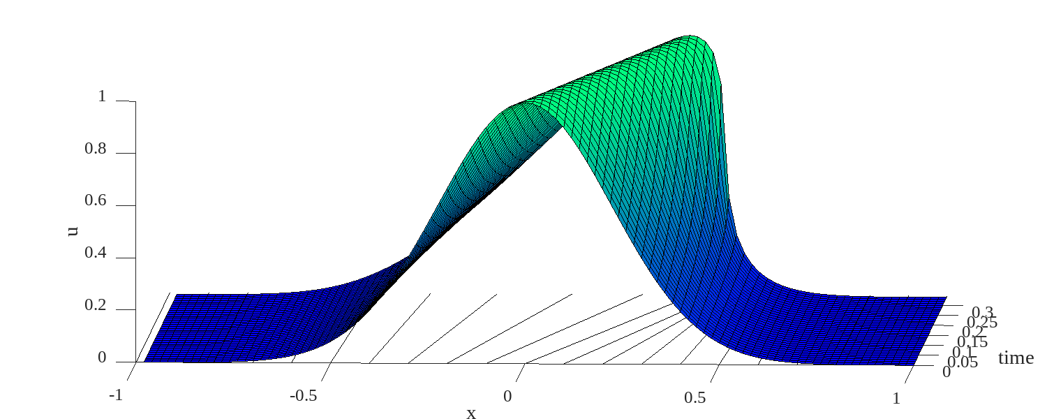
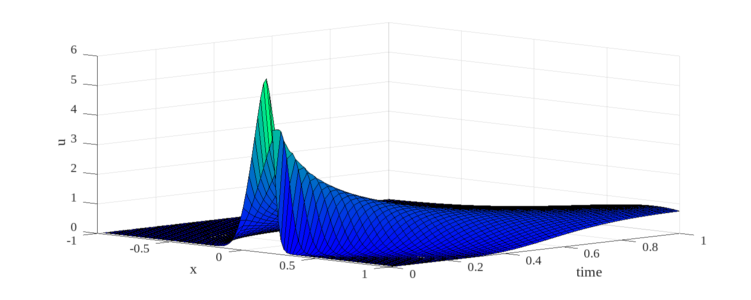
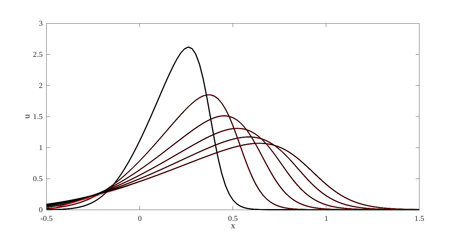
The evolution in time of the velocity from equation 3.41 is illustrated in figure for an initial velocity disturbance $u=\delta(x)$ , at three times. The peak velocity translates toward $+x$ , and the velocity expansion, behind the peak spread out in time. The front, ahead of the peak does not sharpen, because of viscous diffusion.

Figure 3.6: The solution 3.41 as a function of loaction $x$ and time. The solution is omitted for the initial instant since it is a $\delta$ function.

3.2.4 FEM

Now turn our attention to using numerical methods to solve Burgers’ equation. The spatial discretization will be accomplished with FEM. Obtain the weak form by multiplying equation 3.23 by a test function, $\phi_{m}$ and integrate over the domain.

\frac{\partial}{\partial t}\int_{-L}^{L}\!u\,\phi_{m}\;dx+\int_{-L}^{L}\!\left% (u\frac{\partial\,u}{\partial x}\right)\phi_{m}\;dx=\frac{2}{\mbox{Re}}\int_{-% L}^{L}\!\frac{\partial^{2}u}{\partial x^{2}}\phi_{m}\;dx

(3.42)

where we have replaced the infinite domain by a (large enough) domain: $-L\leq x\leq L$ . There needs to be one initial condition and two boundary conditions.

Look for solutions of the form:

u^{t}(x)=\sum_{n=1}^{nx}u^{t}_{n}\phi_{n}

(3.43)

The superscript refers to time and the subscript refers to location.

\frac{\partial}{\partial t}\sum_{n=1}^{nx}\!\int_{-L}^{L}\!\phi_{m}\phi_{n}\,% dx\,u_{n}+\int_{-L}^{L}\!\phi_{m}\sum_{n=1}^{nx}\!\phi_{n}u_{n}\left(\frac{% \partial}{\partial x}\sum_{o=1}^{nx}\!\phi_{o}u_{o}\right)\,dx-\nu\sum_{n=1}^{% nx}\int_{-L}^{L}\!\frac{\partial\phi_{m}}{\partial x}\frac{\partial\,\phi_{n}}% {\partial x}\,dx\,u_{n}=0

(3.44)

or, using matrix notation

\mathcal{M}\frac{\partial\bm{u}}{\partial t}+\left(\mathcal{J}+\nu\,\mathcal{K% }\right)\bm{u}=0.

(3.45)

where $\mathcal{J}$ is itself a function of $\bm{u}$ .

The boundary conditions specify values of the solution at either end of the spatial domain: they aree Dirichlet conditions, similar to the conditions encountered in section LABEL:sec:C2coos. When the interior and boundary portions of equation 3.45 are separated out:

\widetilde{\mathcal{M}}\frac{\partial\widetilde{\bm{u}}}{\partial t}+\left(% \widetilde{\mathcal{J}}+\nu\,\widetilde{\mathcal{K}}\right)\widetilde{\bm{u}}=% -\left(\widehat{\mathcal{J}}+\nu\,\widehat{\mathcal{K}}\right)\widehat{\bm{u}}

(3.46)

where the tilde and hat modifiere are defined in equation 1.41.

Advection

Advection is included as an additional term compared to the linear wave equation, namely

\mathbf{J}=\mathcal{J}\bm{u}=\int_{-L}^{L}\!\phi_{m}\sum_{n=1}^{nx}\!\phi_{n}u% _{n}\left(\frac{\partial}{\partial x}\sum_{o=1}^{nx}\!\phi_{o}u_{o}\right)\,dx

(3.47)

With linear TF, the evaluation of the column vector $\mathbf{J}$ is relatively straightforward, since gradients of the test functions are constant in each elelement. The contribution to node $m$ come from two elements $m$ and $m+1$ , as shown in

\mathbf{J}_{m}=\int_{-L}^{L}\!\phi_{m}\sum_{n=1}^{nx}\!\phi_{n}u_{n}\left(% \frac{\partial}{\partial x}\sum_{o=1}^{nx}\!\phi_{o}u_{o}\right)\,dx

(3.48)

The only contributions come from the interval $x_{m-1}:x_{m+1}$ illustrated in figure 3.7, where $\phi_{m}\neq 0$ .

Figure 3.7: Contributions to the term

\mathbf{J}_{m}

are limited to the interval

x_{m-1}:x_{m+1}

Away from the ends,this allows us to write:

\mathbf{J}_{m}=\int_{x_{m-1}}^{x_{m}}\!\phi_{m}\sum_{n=1}^{nx}\!\phi_{n}u_{n}% \left(\frac{\partial}{\partial x}\sum_{o=1}^{nx}\!\phi_{o}u_{o}\right)\,dx+% \int_{x_{m}}^{x_{m+1}}\!\phi_{m}\sum_{n=1}^{nx}\!\phi_{n}u_{n}\left(\frac{% \partial}{\partial x}\sum_{o=1}^{nx}\!\phi_{o}u_{o}\right)\,dx

(3.49)

\begin{split}\displaystyle\mathbf{J}_{m}=\int_{x_{m-1}}^{x_{m}}\!\phi_{m}\left% (\phi_{m-1}u_{m-1}+\phi_{m}u_{m}\right)\left(\frac{\partial\phi_{m-1}}{% \partial x}u_{m-1}+\frac{\partial\phi_{m}}{\partial x}u_{m}\right)\,dx\\ \displaystyle+\int_{x_{m}}^{x_{m+1}}\!\phi_{m}\left(\phi_{m+1}u_{m+1}+\phi_{m}% u_{m}\right)\left(\frac{\partial\phi_{m+1}}{\partial x}u_{m+1}+\frac{\partial% \phi_{m}}{\partial x}u_{m}\right)\,dx\end{split}

(3.50)

The partial derivatives are constants, either $\pm 1/(\delta x)$ , so the second parenthesis can be moved out of the integral:

\begin{split}\displaystyle\mathbf{J}_{m}=\frac{u_{m}-u_{m-1}}{\delta x}\int_{x% _{m-1}}^{x_{m}}\!\phi_{m}\left(\phi_{m-1}u_{m-1}+\phi_{m}u_{m}\right)\,dx\\ \displaystyle+\frac{u_{m+1}-u_{m}}{\delta x}\int_{x_{m}}^{x_{m+1}}\!\phi_{m}% \left(\phi_{m+1}u_{m+1}+\phi_{m}u_{m}\right)\,dx\end{split}

(3.51)

where $\delta x$ is the distance between neighboring nodes.

\begin{split}\displaystyle\mathbf{J}_{m}=\frac{u_{m}-u_{m-1}}{\delta x}\left(u% _{m-1}\int_{x_{m-1}}^{x_{m}}\!\phi_{m}\phi_{m-1}\,dx+u_{m}\int_{x_{m-1}}^{x_{m% }}\!\phi_{m}^{2}\,dx\right)\\ \displaystyle+\frac{u_{m+1}-u_{m}}{\delta x}\left(u_{m+1}\int_{x_{m}}^{x_{m+1}% }\!\phi_{m}\phi_{m+1}\,dx+u_{m}\int_{x_{m}}^{x_{m+1}}\!\phi_{m}^{2}\,dx\right)% \end{split}

(3.52)

\begin{split}\displaystyle\mathbf{J}_{m}=\left(u_{m}-u_{m-1}\right)\left(\frac% {u_{m-1}}{6}+\frac{u_{m}}{3}\right)+\left(u_{m+1}-u_{m}\right)\left(\frac{u_{m% +1}}{6}+\frac{u_{m}}{3}\right)\\ \displaystyle=\frac{u_{m}u_{m-1}}{6}+\frac{u_{m}^{2}}{3}-\frac{u_{m-1}^{2}}{6}% -\frac{u_{m}u_{m-1}}{3}+\frac{u_{m+1}^{2}}{6}+\frac{u_{m}u_{m+1}}{3}-\frac{u_{% m+1}u_{m}}{6}-\frac{u_{m}^{2}}{3}\end{split}

(3.53)

Finally:

\mathbf{J}_{m}=\frac{1}{6}\left(u_{m+1}^{2}+u_{m}u_{m+1}-u_{m}u_{m-1}-u_{m-1}^% {2}\right)

(3.54)

At the ends:

\mathbf{J}_{1}=\frac{1}{6}(u_{2}-u_{1})(2u_{1}+u_{2}),\quad\mathbf{J}_{n}=% \frac{1}{6}(u_{nx}-u_{nx-1})(2u_{nx}+u_{nx-1})

(3.55)

Noitice that if

\mathcal{J}=\frac{1}{6}\begin{bmatrix}-u_{1}&u_{2}\\ -u_{1}&u_{3}-u_{1}&u_{3}\\ \cdots&\cdots&-u_{m-1}&u_{m+1}-u_{m-1}&u_{m+1}&\cdots\end{bmatrix}

(3.56)

then

\mathbf{J}=\mathcal{J}\bm{u}

(3.57)

Element by element construction

the whole advection term will be $\mathcal{J}\bm{u}$ , where the matrix $\mathcal{J}$ is itself a function of $\bm{u}$ . Element Matrices are $J_{mno}$ .

Time-stepping

Because Burgers’ equation is non-linear, there is no assurance that the stability analysis described earlier in this chapter is pertinent. Instead we compare the stability and accuracy of several methods.

Trapezoidal

\left[\widetilde{\mathcal{M}}+\frac{\delta t}{2}\left(\widetilde{\mathcal{J}}^% {t}+\nu\,\widetilde{\mathcal{K}}\right)\right]\widetilde{\bm{u}}^{t+1}=\left[% \widetilde{\mathcal{M}}-\frac{\delta t}{2}\left(\widetilde{\mathcal{J}}^{t}+% \nu\,\widetilde{\mathcal{K}}\right)\right]\widetilde{\bm{u}}^{t}-\left(% \widehat{\mathcal{J}}^{t}+\nu\,\widehat{\mathcal{K}}\right)\widehat{\bm{u}}

(3.58)

The weakness here is that the matrix $\widetilde{\mathcal{J}}^{t}$ is evaluated at the know time. There is a way to overcome this by using Newton’s method: see Strang page 484.

BDF2

This is a multi step version of the Backward Euler scheme described in section LABEL:sec:C3S2:Acc-Stab. If $u$ is the generic dependent variable, we want to integrate

\frac{\partial u}{\partial t}=f(u,x,t)

(3.59)

where the function $f$ can be non-linear. Instead of using equation LABEL:eq:C3S2:TSBE, we make use of two earlier points:

\frac{3U^{t+1}-4U^{t}+U^{t-1}}{2\,\delta t}=f(U^{t+1},t+1)

(3.60)

For Burgers equation this is:

\left[3\widetilde{\mathcal{M}}+2\delta t\left(\widetilde{\mathcal{J}}^{t}+\nu% \,\widetilde{\mathcal{K}}\right)\right]\widetilde{\bm{u}}^{t+1}=\widetilde{% \mathcal{M}}\left(4\widetilde{\bm{u}}^{t}-\widetilde{\bm{u}}^{t-1}\right)-2% \delta t\left(\widehat{\mathcal{J}}^{t}+\nu\,\widehat{\mathcal{K}}\right)% \widehat{\bm{u}}

(3.61)

A single TR step is taken at first. Then for the second step, values of $U^{t}$ and $U^{t-1}$ are available.

Multi-step: Gadzag

Reference: Time-Differencing Schemes and Transform Methods, J. of Computationa Physics, v 20, 196-207, 1976

This scheme belongs to the predictor-corrector family (Strang pg 486), where a prediction of the new value $U^{t+1}$ is made based on an explicit value of the nonlinear term, then a coorected value is made based on the nonlinear term evaluted based on the predictor. For the Gadzag scheme:

	$\displaystyle U^{t+1}_{p}=U^{t}+\delta t\frac{3\,f^{t}-f^{t-1}}{2}\quad\mbox{% predictor step}$		(3.62)
	$\displaystyle U^{t+1}=U^{t}+\delta t\frac{f^{t}+f^{t+1}_{p}}{2}\quad\mbox{% corrector step}$

where $f^{t+1}_{p}$ is evaluated based on the predictor $U^{t+1}_{p}$ . The Gadzag scheme has the advantage of requiring only one evaluation of matrix $\mathcal{J}$ per time step.

Newton’s method

This method differs conceptually from all other methods described in that it doesn’t explicitly invole an integration in time. Consider

Instead, given the solution at some time, the solution at a later time is found as a correction based on

Each of the four schemes described above has been evaluated by computing the solution to the travelling wave problem described in sectionsec:C3S2:Burgers:TransFront, with $\overline{u}=\delta u=1$ .

Plot comparing ana with different methods

Exercises

1.

Rather than casting the time dependent wave problem as a system of two equations, it can be cast as a single second order system involving the mass and stiffness matrix. Do this for both trapezoidal and leapfrog schemes and compare results to the exact solution and to the two by two system solution.
2.

Evalute several (at least four) integration schemes of your choice to compare their performace as measured by the Infinity norm of the difference between the solution given by the scheme and the exact solution.