Notes on the Finite Element Method 4 Two Dimensional Potential Flows 6 Steady Viscous flow

Chapter 5 Two Dimensional Waves on a Rotating Sheet of Water

5.1 Tides on the $f$ Plane.

5.1.1 Basin, Equations and BC

Consider a thin circular basin of water, of dimensions comparable to an ocean basin, on the $f$ -plane (figure LABEL:Fi:model). The basin consists of a deep region ( $r\leq r_{S}$ ) surrounded by a shallow continental shelf where the depth is $h_{S}$ . Any point in the basin is located by the radius from the center $r$ , the azimuthal position $\theta$ relative to some fixed direction (say, eastward), and by the depth $z$ . The position of the free surface relative to $z=0$ is denoted by $\eta(r,\theta,t)$ . Horizontal dimensions are made non-dimensional by dividing by the basin radius; vertical dimensions are made non-dimensional by dividing by the maximum depth of the basin: for instance the sea level is $\eta=\eta^{*}/H^{*}$ , where $H^{*}$ represents the dimensional maximum depth. Non-dimensional time is the product of time by the forcing frequency. As envisioned here, the basin radius is $4~{}10^{6}~{}m$ , the maximum depth is $4~{}10^{3}~{}m$ , the shelf depth is $10^{2}~{}m$ . The shelf width can range between $4~{}10^{5}~{}m$ and $4~{}10^{4}~{}m$ . The case when there is no shelf is comprehensively treated by Lamb, 1932.

Figure 5.1: Sketch of the model basin. A shelf of depth $h_{s}$ stands between the deeper central portion of the basin and the rim

The problem is governed by the linearized, hydrostatic, shallow water equations. In terms of the non-dimensional variables these are:

\frac{\partial\bm{t}}{\partial t}+\frac{f}{\kappa}\bm{k}\times\bm{t}=-\frac{h}% {\kappa^{2}}\bm{\nabla}(\eta-\overline{\eta})

(5.1)

\frac{\partial\eta}{\partial t}+\bm{\nabla}\bm{\cdot}\bm{t}=0

(5.2)

where $\bm{k}$ is the unit vector pointing along the vertical (out of the page). $\bm{t}=(t^{x},~{}t^{v})$ is the horizontal transport (the product of velocity times depth) vector ( $\bm{t}=\bm{t}^{*}/(\sigma^{*}R^{*}H^{*})$ ), where $\sigma^{*}$ is the dimensional frequency of the forcing. Solutions depend on two non-dimensional parameters: the product of the basin length scale by the shallow water wavenumber in the deep region, $\kappa=\sigma^{*}R^{*}/\sqrt{g^{*}H^{*}}$ , and the ratio of the basin radius to the Rossby radius of deformation, $f=f^{*}R^{*}/\sqrt{g^{*}H^{*}}$ . In the following examples the ratio $f/\kappa$ will be taken to be either $1/2$ , $1$ or $2$ corresponding to superinertial, inertial of subinertial forcing. The radius of basins of interest here, is comparable to the shallow water wavelength, so $\kappa\mathcal{O}(1)$ .

The boundary conditions specify that the transport normal to the boundary ( $\bm{t}\cdot\bm{n}$ ) must be zero at the boundary ( $r=1$ ). If the bottom depth varies, as in the case of a step continental shelf, matching conditions at the slope break ( $r=r_{S}$ ) require that both the sea level and the transport normal to the shelf break be the same in each region.

Equations 5.1 and 5.2 can be combined into a single equation for $\eta$ as follows: after some manipulation equation 5.1 can be writen as:

\frac{\partial^{2}\bm{t}}{\partial t^{2}}+\frac{f}{\kappa}\bm{k}\times\frac{% \partial\bm{t}}{\partial t}-\frac{f}{\kappa}\bm{k}\times\frac{\partial\bm{t}}{% \partial t}+\frac{f^{2}}{\kappa^{2}}\bm{t}=-\frac{h}{\kappa^{2}}\bm{\nabla}% \left(\frac{\partial(\eta-\overline{\eta})}{\partial t}\right)+\frac{f\,h}{% \kappa^{3}}\bm{k}\times\bm{\nabla}(\eta-\overline{\eta})

(5.3)

or:

\frac{\partial^{2}\bm{t}}{\partial t^{2}}+\frac{f^{2}}{\kappa^{2}}\bm{t}=-% \frac{h}{\kappa^{2}}\bm{\nabla}\left(\frac{\partial(\eta-\overline{\eta})}{% \partial t}\right)+\frac{f\,h}{\kappa^{3}}\bm{k}\times\bm{\nabla}(\eta-% \overline{\eta})

(5.4)

Next write equation 5.2 as:

\frac{\partial}{\partial t}\left(\frac{\partial^{2}\eta}{\partial t^{2}}+\frac% {f^{2}}{\kappa^{2}}\eta\right)+\bm{\nabla}\bm{\cdot}\left(\frac{\partial^{2}% \bm{t}}{\partial t^{2}}+\frac{f^{2}}{\kappa^{2}}\bm{t}\right)=0

(5.5)

Substituting equation 5.4 gives:

\frac{\partial}{\partial t}\left(\frac{\partial^{2}\eta}{\partial t^{2}}+\frac% {f^{2}}{\kappa^{2}}\eta\right)+\bm{\nabla}\bm{\cdot}\left(-\frac{h}{\kappa^{2}% }\bm{\nabla}\left(\frac{\partial(\eta-\overline{\eta})}{\partial t}\right)+% \frac{f\,h}{\kappa^{3}}\bm{k}\times\bm{\nabla}(\eta-\overline{\eta})\right)=0

(5.6)

The time dependence is dealt with by confining attention to solutions that are periodic in time at the forcing frequency. Capitalized symbols refer to the time-independent amplitude and phase of the corresponding variable. New dependent variables are defined as:

\eta(\bm{x},t)=\mbox{Re}{[N(\bm{x})\mathrm{e}^{-\mathrm{i}\,t}]}\quad\bm{t}=% \mbox{Re}{[\bm{T}(\bm{x})\mathrm{e}^{-\mathrm{i}\,t}]}

(5.7)

where the new variables $N$ and $T$ are complex, and $\bm{x}$ is the two dimensional coordinate vector (in whatever coordinate system is convenient given the geometry of the problem). In terms of these new variables, the mass conservation equation 5.2 is:

-\mathrm{i}N+\bm{\nabla}\bm{\cdot}\bm{T}=0

(5.8)

The horizontal momentum equation 5.1 yields the following expression for the transport:

(\kappa^{2}-f^{2})\bm{T}=-h\left(\mathrm{i}\bm{\nabla}N^{\prime}-\frac{f}{% \kappa}\bm{k}\times\bm{\nabla}N^{\prime}\right)

(5.9)

where the sea level anomaly from the equilibrium tide, $N^{\prime}=N-\overline{N}$ , has been introduced for convenience. This is used to eliminate transport from equation 5.8:

\bm{\nabla}\bm{\cdot}\left[h\left(\bm{\nabla}N^{\prime}+\mathrm{i}\frac{f}{% \kappa}\bm{k}\times\bm{\nabla}N^{\prime}\right)\right]+(\kappa^{2}-f^{2})N=0;% \quad\bm{T}\cdot\bm{n}=0.

(5.10)

For the boundary conditions, the transport (equation 5.9 normal to the boundary has to be zero at a closed boundary. This is a boundary condition on the derivative of the sea level: a Neumann condition. At an open boundary, the sea level has to be specified.

In cartesian coordinates the governing equation 5.10 becomes :

\frac{\partial}{\partial x}\left(h\frac{\partial N^{\prime}}{\partial x}\right% )+\frac{\partial}{\partial y}\left(h\frac{\partial N^{\prime}}{\partial y}% \right)+\frac{\mathrm{i}f}{\kappa}\left[\frac{\partial}{\partial x}\left(h% \frac{\partial N^{\prime}}{\partial y}\right)-\frac{\partial}{\partial y}\left% (h\frac{\partial N^{\prime}}{\partial x}\right)\right]+(\kappa^{2}-f^{2})\,N^{% \prime}=(f^{2}-\kappa^{2})\overline{N}

(5.11)

with

\mathrm{i}\frac{\partial N^{\prime}}{\partial x}-\frac{f}{\kappa}\frac{% \partial N^{\prime}}{\partial y}=0\;\mbox{at}\;x=\pm 1;\quad\mathrm{i}\frac{% \partial N^{\prime}}{\partial y}+\frac{f}{\kappa}\frac{\partial N^{\prime}}{% \partial x}=0\;\mbox{at}\;\tilde{y}=\pm 1

(5.12)

In this form, the terms on the right only involve $N^{\prime}$ , and the right hand side is the forcing term: this is a non-homogeneous PDE for $N^{\prime}$ .

In polar coordinates:

\frac{\partial}{\partial r}\left(r\,h\frac{\partial N^{\prime}}{\partial r}% \right)+\frac{\partial}{\partial\theta}\left(\frac{h}{r}\frac{\partial N^{% \prime}}{\partial\theta}\right)+\frac{\mathrm{i}f}{\kappa}\left(\frac{\partial h% }{\partial r}\frac{\partial N^{\prime}}{\partial\theta}-\frac{\partial h}{% \partial\theta}\frac{\partial N^{\prime}}{\partial r}\right)+(\kappa^{2}-f^{2}% )\,r\,N^{\prime}=(f^{2}-\kappa^{2})\,r\,\overline{N}

(5.13)

The normal transport vanishes along the boundary of the basin:

\mathrm{i}\frac{\partial N^{\prime}}{\partial r}-\frac{f}{\kappa r}\frac{% \partial N^{\prime}}{\partial\theta}=0\quad\mbox{at}\quad r=1.

(5.14)

Axisymmetric circular basins.

In polar coordinates equation 5.10 is

	$\displaystyle\frac{\partial}{\partial\theta}\left(\frac{h}{r}\frac{\partial N^% {\prime}}{\partial\theta}\right)+\frac{\partial}{\partial r}\left(rh\frac{% \partial N^{\prime}}{\partial r}\right)$	$\displaystyle+$	$\displaystyle\frac{\mathrm{i}f}{\kappa}\left(\frac{\partial h}{\partial r}% \frac{\partial N^{\prime}}{\partial\theta}-\frac{\partial h}{\partial\theta}% \frac{\partial N^{\prime}}{\partial r}\right)$		(5.15)
	$\displaystyle+(\kappa^{2}-f^{2})\,r\,N^{\prime}$	$\displaystyle=$	$\displaystyle(f^{2}-\kappa^{2})\,r\,\overline{N}$

The normal transport vanishes along the boundary of the basin:

\mathrm{i}\frac{\partial N^{\prime}}{\partial r}-\frac{f}{\kappa r}\frac{% \partial N^{\prime}}{\partial\theta}=0\quad\mbox{at}\quad r=1.

(5.16)

Lamb’s Solution

Lamb (1932) has shown that if $h=1$ and if the equilibrium tide can be expressed as $\overline{N}=r^{|m|}\mathrm{e}^{\mathrm{i}m\theta}$ , the equation governing $N$ is:

\frac{\partial}{\partial r}\left(r\frac{\partial N}{\partial r}\right)+\frac{1% }{r}\frac{\partial^{2}N}{\partial\theta^{2}}+(\kappa^{2}-f^{2})r\,N=0,\quad% \frac{\partial N}{\partial r}+\mathrm{i}\frac{f}{\kappa r}\frac{\partial N}{% \partial\theta}=\frac{\partial\overline{N}}{\partial r}+\mathrm{i}\frac{f}{% \kappa r}\frac{\partial\overline{N}}{\partial\theta}=|m|-m\frac{f}{\kappa}\;% \mbox{at}\;r=1.

(5.17)

Separate variables as $N(r,\theta)=R(r)\Theta(\theta)$ . The azimuthal component is $\mathrm{e}^{\mathrm{i}m\theta}$ . Then the radial component $R$ is the solution to:

\frac{d}{dr}\left(r\frac{dR}{dr}\right)+\left(\kappa^{2}-f^{2}-\frac{m^{2}}{r^% {2}}\right)r\,R=0,\quad\frac{dR}{dr}-m\frac{f}{\kappa}\frac{R}{r}=|m|-m\frac{f% }{\kappa}\;\mbox{at}\;r=1.

(5.18)

This is Bessel’s equation (if $\kappa\geq f$ ), or the modified Bessel’s equation otherwise. The amplitude of the response is determined by the boundary condition. Bessel function derivatives are:

\frac{d\,\mathrm{J}_{m}(\alpha r)}{dr}=-\alpha\mathrm{J}_{m+1}(\alpha r)+\frac% {m}{r}\mathrm{J}_{|m|}(\alpha r);\quad\frac{d\,\mathrm{I}_{|m|}(\alpha r)}{dr}% =\alpha\mathrm{J}_{m+1}(\alpha r)+\frac{m}{r}\mathrm{J}_{|m|}(\alpha r)

(5.19)

So long as $\kappa>f$ , the solution for $N$ is:

N(r,\theta)=\frac{(|m|-f\,m/k)\mathrm{J}_{|m|}(\alpha\,r)}{(|m|-f\,m/k)\mathrm% {J}_{m}(\alpha)-\alpha\mathrm{J}_{|m|+1}(\alpha)}\mathrm{e}^{\mathrm{i}m\theta% },\quad\mbox{where}\quad\alpha=\sqrt{\kappa^{2}-f^{2}}

(5.20)

If $\kappa=f$

N(r,\theta)=\begin{cases}\overline{N}(r,\theta)=r^{|m|}\mathrm{e}^{\mathrm{i}m% \theta}&\text{if $m<0$}\\ \frac{m(m+1)}{(m(m+1)-f^{2})}r^{|m|}\mathrm{e}^{\mathrm{i}m\theta}&\text{if $m% >0$}\end{cases}

(5.21)

For $\kappa<f$ The solution is

N(r,\theta)=\frac{(|m|-f\,m/k)\mathrm{I}_{|m|}(\alpha\,r)}{(|m|-f\,m/k)\mathrm% {I}_{m}(\alpha)+\alpha\mathrm{I}_{{m}+1}(\alpha)}\mathrm{e}^{\mathrm{i}m\theta% },\quad\mbox{where}\quad\alpha=\sqrt{f^{2}-\alpha^{2}}

(5.22)

The solutions are illustrated in figure 5.2.

Figure 5.2: Amplitude and phase of the sea level $N$ in a basin forced by $\overline{N}=r^{|m|}\mathrm{e}^{\mathrm{i}\,m\,\theta}$ .

These solutions can be extended to axisymmetric circular domains where a shelf-like rim separated the central deep region from the boundary, as illustrated in figure 5.1. It is also possible, by using Green’s functions, to find the response of an axisymmetric basin to forcing that propagates across the domain as a wave travelling from east to west, consistent with the equilibrium tide at mid-latitudes. Four examples of these solutions are illustrated in figure LABEL:Fi:EWAnalytic.

5.2 Finite Element Method

5.2.1 Weak Form

The weak form of equation 5.10 is obtained in the usual way:

(\kappa^{2}-f^{2})\int\!\phi_{m}\bm{\nabla}\bm{\cdot}\bm{T}\,da-\mathrm{i}(% \kappa^{2}-f^{2})\int\!\phi_{m}N^{\prime}\,da=\mathrm{i}(\kappa^{2}-f^{2})\int% \!\phi_{m}\overline{N}\,da;

(5.23)

division by $\kappa^{2}-f^{2}$ is avoided so as to not exclude the possibility that $f=\pm\kappa$ . The transport is as given in equation 5.9. Integrate the first term of equation 5.23 by parts:

\int\!\phi_{m}\bm{\nabla}\bm{\cdot}\bm{T}\,da=\int\!\bm{\nabla}\bm{\cdot}(\phi% _{m}\bm{T})\,da-\int\!\bm{T}\bm{\cdot}\bm{\nabla}{\phi_{m}}\,da

(5.24)

The divergence theorem is:

\int_{A}\!\bm{\nabla}\bm{\cdot}\bm{U}da=\int_{S}\bm{U}.\bm{n}\,ds

(5.25)

where $\bm{U}$ is any arbitrary vector, $S$ represents the boundary of the domain $A$ and $\bm{n}$ is the unit normal to $S$ . Equation 5.23 becomes:

(f^{2}-\kappa^{2})\int\!\bm{\nabla}\phi_{m}\bm{\cdot}\bm{T}\,da-\mathrm{i}(% \kappa^{2}-f^{2})\int\!\phi_{m}N^{\prime}\,da+\mathrm{i}(\kappa^{2}-f^{2})\int% \!\phi_{m}\overline{N}\,da=-\mathrm{i}h(f^{2}-\kappa^{2})\int_{S}\bm{T}.\bm{n}% \,ds

(5.26)

The boundary condition states that the transport normal to a boundary is zero, so the integral on the right of equation 5.26 is equal to zero. quation 5.23 becomes:

(f^{2}-\kappa^{2})\int\!\bm{\nabla}\phi_{m}\bm{\cdot}\bm{T}\,da-\mathrm{i}(% \kappa^{2}-f^{2})\int\!\phi_{m}N^{\prime}\,da=-\mathrm{i}(f^{2}-\kappa^{2})% \int\!\phi_{m}\overline{N}\,da

(5.27)

The tranport is related to $N^{\prime}$ by equation 5.9: the transport can be eliminated from equation 5.27. In cartesian coordinates equation 5.27 is:

\begin{split}\displaystyle\int\!\left[h\left(\frac{\partial\phi_{m}}{\partial x% }\frac{\partial\,N^{\prime}}{\partial x}+\frac{\partial\phi_{m}}{\partial y}% \frac{\partial\,N^{\prime}}{\partial y}\right)+\mathrm{i}\frac{f\,h}{\kappa}% \left(\frac{\partial\phi_{m}}{\partial x}\frac{\partial\,N^{\prime}}{\partial y% }-\frac{\partial\phi_{m}}{\partial y}\frac{\partial\,N^{\prime}}{\partial x}% \right)\right]\,da\\ \displaystyle+(\kappa^{2}-f^{2})\int\!\phi_{m}N^{\prime}\,da=(f^{2}-\kappa^{2}% )\int\!\phi_{m}\overline{N}\,da\end{split}

(5.28)

Look for the solution as an expansion in terms of the trial functions:

N^{\prime}(x,y)=\sum_{n=1}^{N}\!N^{\prime}_{n}\phi_{n}(x,y)

(5.29)

where $N^{\prime}_{n}$ represent the value of the solution at each node. Withis substitution, the weak form becomes:

\begin{split}\displaystyle\sum_{n=1}^{N}\int\!\left[h\left(\frac{\partial\phi_% {m}}{\partial x}\frac{\partial\,\phi_{n}}{\partial x}+\frac{\partial\phi_{m}}{% \partial y}\frac{\partial\,\phi_{n}}{\partial y}\right)+\mathrm{i}\frac{f\,h}{% k}\left(\frac{\partial\phi_{m}}{\partial x}\frac{\partial\,\phi_{n}}{\partial y% }-\frac{\partial\phi_{m}}{\partial y}\frac{\partial\,\phi_{n}}{\partial x}% \right)\right]\,da\\ \displaystyle+(\kappa^{2}-f^{2})\sum_{n=1}^{N}\int\!\phi_{m}\phi_{n}\,da=(f^{2% }-\kappa^{2})\int\!\phi_{m}\overline{N}\,da\end{split}

(5.30)

Equation 5.30 is a system of $N$ equations in the $N$ unknowns $N^{\prime}_{n}$ . Using matrix notation it can be written as

\left[(\kappa^{2}-f^{2})\mathcal{M}-\mathcal{L}\right]\,\bm{N^{\prime}}=\bm{F}

(5.31)

where $\bm{N^{\prime}}$ represents the solution column vector, and $\mathcal{M}$ is the usual mass matrix with elements

M_{mn}=\int_{A}\!\phi_{m}\phi_{n}\,da

(5.32)

L_{mn}=\int_{A}\!\left[h\left(\frac{\partial\phi_{m}}{\partial x}\frac{% \partial\,\phi_{n}}{\partial x}+\frac{\partial\phi_{m}}{\partial y}\frac{% \partial\,\phi_{n}}{\partial y}\right)+\mathrm{i}\frac{f\,h}{\kappa}\left(% \frac{\partial\phi_{m}}{\partial x}\frac{\partial\,\phi_{n}}{\partial y}-\frac% {\partial\phi_{m}}{\partial y}\frac{\partial\,\phi_{n}}{\partial x}\right)% \right]\,da

(5.33)

is a special version of the stiffness matrix, and the load vector elements are

F_{m}=-\kappa^{2}\int_{A}\!\mathrm{e}^{-\mathrm{i}k\,x}\phi_{m}\,da

(5.34)

5.2.2 Constant, or slowly varying depth

If the depth $h=1$ is constant the special stiffness matrix can be written

L_{mn}=K_{mn}+\mathrm{i}\frac{f}{k}\,O_{mn}

(5.35)

where $K_{mn}$ represents the elements of the ususal stiffness matrix and

O_{m,n}=\int_{A}\!\left(\frac{\partial\phi_{m}}{\partial x}\frac{\partial\,% \phi_{n}}{\partial y}-\frac{\partial\phi_{m}}{\partial y}\frac{\partial\,\phi_% {n}}{\partial x}\right)\,da

(5.36)

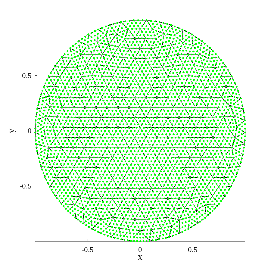
5.2.3 Discretizing the Domain: the Grid.

A typical circular grid suitable for cubic TF is illustrated in figure 5.4.

Typical grid for solving PDEs in a circular region. The
mesh is shown as black lines. Cubic TF require ten nodes in each
element. The nodes are shown as green circles. (Grid XTHFC3067) — Figure 5.4: Typical grid for solving PDEs in a circular region. The mesh is shown as black lines. Cubic TF require ten nodes in each element. The nodes are shown as green circles. (Grid XTHFC3067)

5.2.4 Assembly

Constant Depth

Element Matrices

For cubic polynomials, there are ten TF on each element. Each TF is unity at a single node, and zero at the nine other positions. The TF are as defined in the second equality in equation LABEL:eq:C4S1:defTF. The coefficients for the polynomials are obtained following the method described in section LABEL:sec:C4S1:LTF.

Given $\mathcal{C}$ , the matrix of coefficients (see section LABEL:sec:C4S1:LTF), The element load vector $\bm{Fe}$ is determined as follows:

Fe_{m}=\sum_{k=1}^{10}C_{k,m}\!\int_{A}\!x^{p(k)}y^{q(k)}\,dx\,dy

(5.37)

where for cubic polynomials, the exponents $p$ and $q$ are listed in table 5.1.

k	1	2	3	4	5	6	7	8	9	10
p(k)	0	1	0	2	1	0	3	2	1	0
q(k)	0	0	1	0	1	2	0	1	2	3

Table 5.1: Powers

p, q

as a function of

k

for Cubic TF.

First determine the column vector $\bm{I}^{F}$ whose elements are

I^{F}_{k}=\int_{A}\!x^{p(k)}y^{q(k)}\,dx\,dy=c^{q+1}\frac{[a^{p+1}-(-b)^{p+1}]% p!q!}{(p+q+2)!}

(5.38)

where $a$ , $b$ and $c$ are defined in figure LABEL:Fi:C4S12triangles. Then

\bm{Fe}=\mathcal{C}^{T}\bm{I}^{F}

(5.39)

The mass element matrix is evaluated in similar fashion, starting from

Me_{m,n}=\sum_{k=1}^{10}C_{k,m}\sum_{l=1}^{10}C_{l,n}\!\int_{A}\!x^{p(k)+p(l)}% y^{q(k)+q(l)}\,dx\,dy

(5.40)

Begin by forming the $10\times 10$ matrix $\mathcal{I}^{M}$ with elements

I^{M}_{k,l}=\int_{A}\!x^{p(k)+p(l)}y^{q(k)+q(l)}\,dx\,dy=c^{q(k)+q(l)+1}\frac{% [a^{p(k)+p(l)+1}-(-b)^{p(k)+p(l)+1}]p(k)+p(l)!q(k)+q(l)!}{(p(k)+p(l)+q(k)+q(l)% +2)!}

(5.41)

To vectorize, in Octave form two $10\times 10$ matrices, P and Q as follows:

  P=repmat(p,kcubic,1)+repmat(p’,1,kcubic);
  Q=repmat(q,kcubic,1)+repmat(q’,1,kcubic);
  %% get Me
  IsupM=c.^(Q+1).*(a.^(P+1)-(-b).^(P+1)).*factorial(P).*factorial(Q)./factorial(P+Q+2);
  Me=transpose(C)*IsupM*C;

The element mass matrix is then:

\mathcal{M}e=\mathcal{C}^{T}\mathcal{I}^{M}\mathcal{C}

(5.42)

Similar expressions are fount for the two element stiffness matrices $\mathcal{K}e$ and $\mathcal{O}e$ .

Variable Depth

If the depth varies two courses of action are possible: the first consists in moving the depth term, $h$ outside of the integral in, for instance, the first term in equation 5.30. The second approach is to determine the required matrix, say the stiffness using quadrature as follows:

for kq=1:length(wt); %quadrature loop
  xv=x1*(1-xq(kq)-yq(kq))+x2*xq(kq)+x3*yq(kq);
  yv=y1*(1-xq(kq)-yq(kq))+y2*xq(kq)+y3*yq(kq);
  rv=sqrt(xv^2+yv^2);
  hv=1;
  if rv>1-Ls
    hv=hs;
  endif
  phi_x=(p.*xq(kq).^(p-1).*yq(kq).^q)*C;
  phi_y=(q.*xq(kq).^p.*yq(kq).^(q-1))*C;
  phi_X=[phi_x’,phi_y’]*G;
  for m=1:10
    for n=1:10
      Ke(m,n)=Ke(m,n)+wt(kq)*hv*(phi_X(m,1)*phi_X(n,1)+phi_X(m,2)*phi_X(n,2));
      Oe(m,n)=Oe(m,n)+wt(kq)*hv*(phi_X(m,1)*phi_X(n,2)-phi_X(m,2)*phi_X(n,1));
    endfor
  endfor
endfor
Ke=Ke*Area;
Oe=Oe*Area;