Notes on the Finite Element Method 3 Time-dependent Waves and Burgers’ Equation 5 Two Dimensional Waves on a Rotating Sheet of Water

Chapter 4 Two Dimensional Potential Flows

4.1 Equations and Boundary Conditions

4.1.1 Potential and Stream functions.

Begin with the mass conservation equation:

\nabla\cdot\mathbf{u}=0

(4.1)

Because the curl of the gradient of any scalar function has to be zero, if the vorticity vector $\bm{\omega}$ defined as

\bm{\omega}=\nabla\times\mathbf{u}=0

(4.2)

the velocity can be defined as the gradient of a scalar potential function:

\mathbf{u}=\nabla\phi

(4.3)

then the governing equation for $\phi$ comes directly from continuity:

\nabla\cdot\nabla\phi=\nabla^{2}\phi=0

(4.4)

This is the simplest possible elliptic pde: Laplace’s equation. Since there can be no flow through a boundary, the required boundary conditions are that the normal component of $\phi$ vanish at the boundary. These are neumann conditions.

For a two dimensional flow (can be extended to axisymmetric) flow, a streamfunction can be defined as:

u=-\frac{\partial\psi}{\partial y};\quad v=\frac{\partial\psi}{\partial x}

(4.5)

In general, the streamfunction is related to the vorticity by:

\nabla^{2}\psi=-\bm{\omega}

(4.6)

The condition that the vorticity be zero then gives:

\nabla^{2}\psi=0

(4.7)

so that both the stream and potential functions satisfy Laplace’s equation. This is very surprising. Usually the combined NS and mass conservation equations have to be solved for the velocities and pressure. Now a single (very simple) equation has to be solved for a single dependent variable: the potential function, or the streamfunction.. Part of the mystery is wrapped up in the condition that the vorticity has to be zero. For completeness, consider how to evaluate the pressure field given the potential $\phi$ ..

4.1.2 The Bernouilli Equation

Once the streamfunction or the potential function is know, the velocities are given by either equation 4.3, or equation 4.5. The pressure is then given by Bernouilli’s equation. The momentum equation (now called the Euler equation) can be written as:

\frac{\partial\mathbf{u}}{\partial t}+(\mathbf{u}\cdot\nabla)\mathbf{u}=-\frac% {\nabla p}{\rho}+\mathbf{g}

(4.8)

Noting that

(\mathbf{u}\cdot\nabla)\mathbf{u}=\frac{1}{2}\nabla(u^{2})-\mathbf{u}\times% \nabla\times\mathbf{u}

(4.9)

and with $\bm{\omega}=\nabla\times\mathbf{u}=0$ , for a constant density fluid, the momentum equation is

\frac{\partial\mathbf{u}}{\partial t}+\frac{1}{2}\nabla(u^{2})-\mathbf{u}% \times\bm{\omega}=-\frac{1}{\rho}\nabla(p+\rho gz)

(4.10)

This is Bernouilli’s equation. The component parallel to a streamline (or to $\mathbf{u}$ ) is:

\frac{\partial u}{\partial t}+\frac{\partial}{\partial s}\left(\frac{1}{2}u^{2% }+\frac{p}{\rho}+gz\right)=0

(4.11)

where $s$ represents distance along a streamline. This is because $\bm{\omega}$ is perpendicular to $\mathbf{u}$ . The component normal to the streamline is:

u\frac{\partial v}{\partial s}=-\frac{1}{\rho}\frac{\partial(p+\rho gz)}{% \partial n}

(4.12)

which shows that for a flow to change direction, the pressure must vary in the direction normal to the streamline.

For steady flow, the inviscid momentum equation can be integrated between any points on a streamline with the result that

\frac{1}{2}u^{2}+\frac{p}{\rho}+gz=B(\psi)

(4.13)

in words, the expression on the left hand side is a constant along the streamline. This is Bernouilli’s equation for steady, inviscid, rotational flow. The finite element method is ideally suited for such problems in two dimensions, particularly when the domain is irregular.

4.2 Grids

4.2.1 DistMesh

Read Strang pp 305-316
Mesh regularity is a desirable property for Finite Elements. By regularity we don’t mean size, what we are looking for are grids where there are no long, skinny triangles. Ideally the grid would consist only of equlqteral triangles. Persson wrote DistMesh with this goal in mind. Three grids produced by DistMesh are illustrated in figure 4.1.

Different grids produced by DistMesh. Left: simple
rectangular gria; center: circle in a rectangle; right: same with
progressively varying mesh size. — Figure 4.1: Different grids produced by DistMesh. Left: simple rectangular gria; center: circle in a rectangle; right: same with progressively varying mesh size.

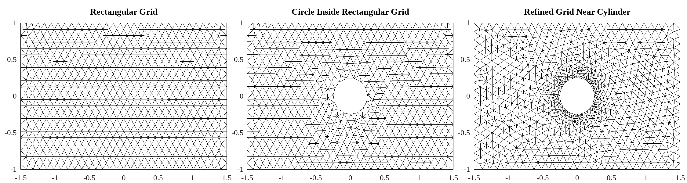
Each mesh consists of $M$ nodes. The gridding procedure determines coordinates for each node as well as a connection table consisting of a list of the three nodes at the vertex of each element.

The script to produce these plots is listed in 4.5.1

4.2.2 Trial Functions and Elements

Just as in the one-dimensional case, the test function is defined as having unit value at one particular node, and zero at all other nodes. A test function is illustrated in figure 4.2.

A single linear test function. The value is non-zero at a
single node of the grid. Each of the slanting sides is one
element. If the elements were all equilateral, they would always
be six elements contributing to each TF. — Figure 4.2: A single linear test function. The value is non-zero at a single node of the grid. Each of the slanting sides is one element. If the elements were all equilateral, they would always be six elements contributing to each TF.

It is teepee shaped, the central node is directly connected to six peripheral nodes: the functions has six sides, or elements.

Test and Trial Functions

As in the one-dimensional case, there are several choices for the polynomial representing the test (or trial) function in an element. The FEM procedure (Galerkin’s method) consists of representing the dependent variable (e.g. $u(x,y)$ ) as an expansion over a set of test functions $\phi_{m}(x,y)$ , in such a way that the governing equation and BC provide estimates of the solution at each node. The test functions are always chosen to be polynomials:

u(x,y)=\sum_{m=1}^{M}\!u_{m}\phi_{m}(x,y)\quad\mbox{where}\quad\phi_{m}=\sum_{% k=1}^{K}\!C_{k,m}x^{p(k)}y^{q(k)}

(4.14)

The constant $u_{m}$ is the value of the solution at node $m$ .

Linear Test Functions

The simplest representation uses linear polynomials. The most general form for a two dimensional test function is $\phi_{m}(x,y)=C_{1,m}+C_{2,m}\,x+C_{3,m}\,y$ . This conforms to equation 4.14 with $k$ , $p$ and $q$ related as in table 4.1.

k	1	2	3
p(k)	0	1	0
q(k)	0	0	1

Table 4.1: Powers

p, q

as a function of

k

for Linear TF.

Each triangular element requires three TF, corresponding to the maximum value occuring at each of the three vertices.

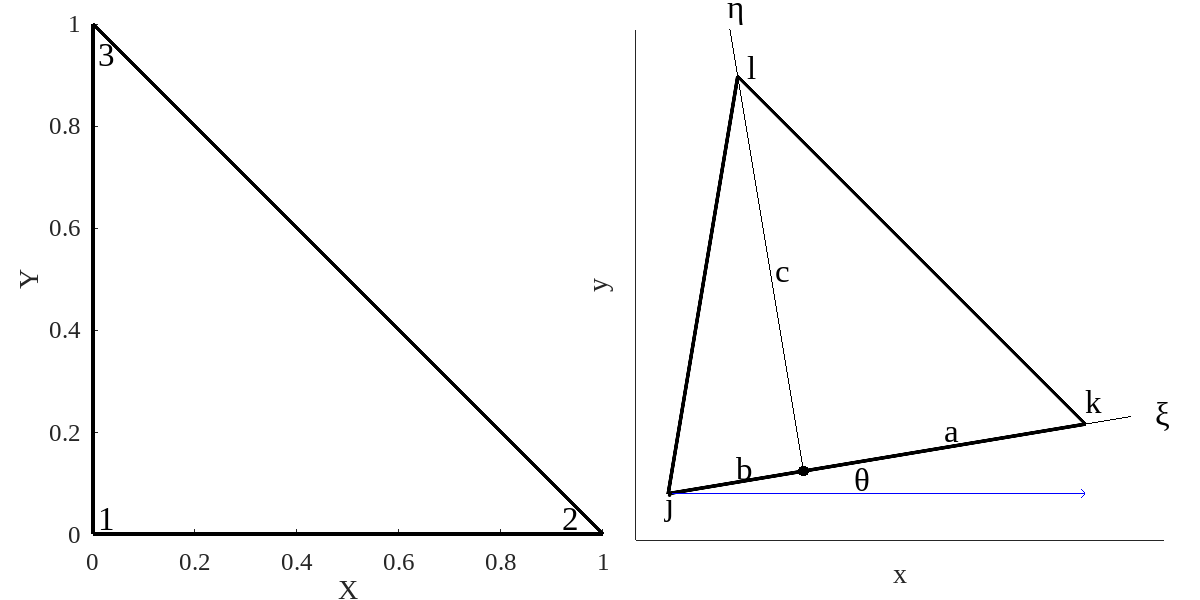
The general approach to finding the coefficients in equation 4.14 is to write a system of equations that satisfies the constraint that each TF is unity at a vertex and zero at the three other vertices. A reference element, known as the canonical triangle, with coordinates $0,0$ ; $1,0$ ; and $0,1$ is illustrated in the left frame of figure 4.3.

Elements of a test function. Left: the canonical triangle.
The bold set numbers identify the locations where each trial
function is 1. Right: an arbitrary triangle (In Cowper’s
notation). — Figure 4.3: Elements of a test function. Left: the canonical triangle. The bold set numbers identify the locations where each trial function is 1. Right: an arbitrary triangle (In Cowper’s notation).

For this example, the three equations for $\phi_{1}$ are:

$\displaystyle C_{11}$	$\displaystyle=$	$\displaystyle 1,\quad\phi_{1}\,@\,(0,0)$	(4.15)
$\displaystyle C_{11}+C_{21}$	$\displaystyle=$	$\displaystyle 0,\quad\phi_{1}\,@\,(0,1)$
$\displaystyle C_{11}+C_{31}$	$\displaystyle=$	$\displaystyle 0,\quad\phi_{1}\,@\,(1,0)$

The solution is: $C_{11}=1$ , $C_{21}=-1$ and $C_{31}=-1$

This approach may be extended to all three test functions in one step by writing:

\mathcal{T}\mathcal{C}=\mathcal{I}\quad\mbox{or, explicitly:}\quad\begin{% bmatrix}1&0&0\\ 1&1&0\\ 1&0&1\end{bmatrix}\begin{bmatrix}C_{11}&C_{12}&C_{13}\\ C_{21}&C_{22}&C_{23}\\ C_{31}&C_{32}&C_{33}\end{bmatrix}=\begin{bmatrix}1&0&0\\ 0&1&0\\ 0&0&1\end{bmatrix}

(4.16)

$\mathcal{T}$ is made up of the values $1,x,y$ at each of the three nodes. Then $\mathcal{C}=\mathcal{T}^{-1}$ is the matrix of coefficients. In this case

\mathcal{C}=\begin{bmatrix}C_{11}&C_{12}&C_{13}\\ C_{21}&C_{22}&C_{23}\\ C_{31}&C_{32}&C_{33}\end{bmatrix}=\begin{bmatrix}1&0&0\\ -1&1&0\\ -1&0&1\end{bmatrix}

(4.17)

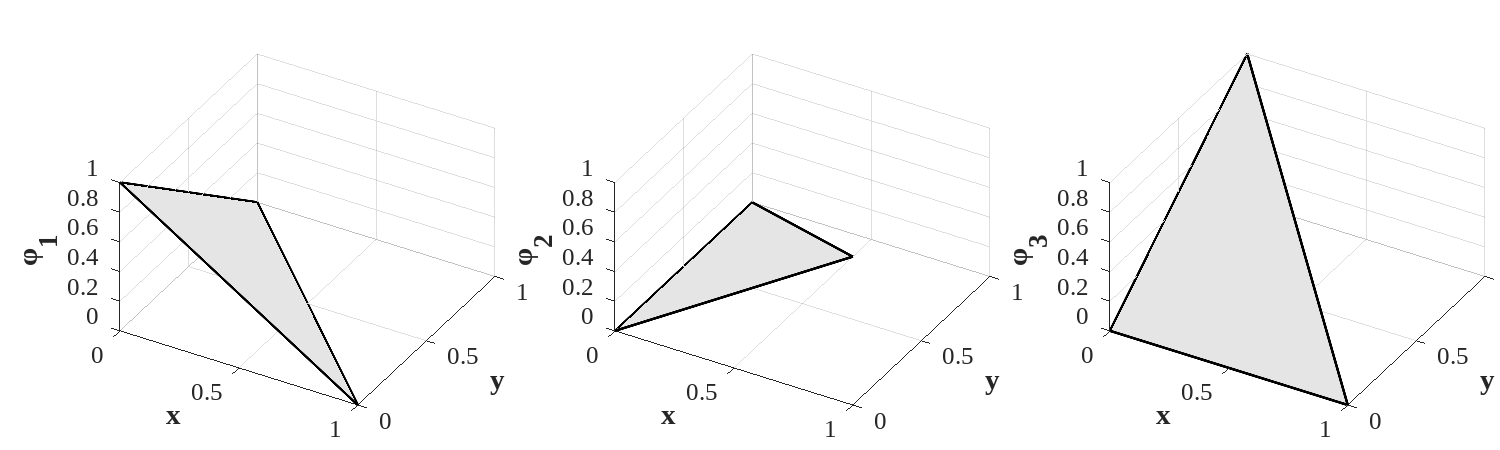
For the canonical triangle, the three test functions are therefore:

\phi_{1}=1-X-Y,\quad\phi_{2}=X,\quad\phi_{3}=Y.

(4.18)

These 3 functions are illustrated in figure 4.4.

Figure 4.4: The three linear test functions in the canonical triangle.

Other choices of test functions include quadratic and cubic Legendre polynomials and quintic Hermite polynomials.

For the general triangle illustrated on the right of figure 4.3. The coordinates of each vertex are given in table 4.2.

Vertex	$x$	$y$
$j$	$0.1$	$0.1$
$k$	$1$	$0.25$
$l$	$0.25$	$1$

Table 4.2: Vertex coordinates for the general triangle illustrated on the right of figure 4.3.

The matrices $\mathcal{T}$ and $\mathcal{C}$ are:

\mathcal{T}=\begin{bmatrix}1&-b&0\\ 1&a&0\\ 1&0&c\end{bmatrix};\quad\mathcal{C}=\frac{1}{bc+ac}\begin{bmatrix}ac&bc&0\\ -c&c&0\\ -a&-b&a+b\end{bmatrix}

(4.19)

4.3 The Stream Function

If the velocity is solenoidal (meaning the velocity satisifies $\bm{\nabla}\times\bm{u}=\bm{\omega}=0$ ), the velocity can be written as the gradient of a potential function $\varphi(x,y)$ ¹¹ 1 please do not confuse the potential function $\varphi$ with the test functions $\phi$ . For two dimensional flow, a streamfunction $\psi(x,y)$ may also be defined. The streamfunction is related to the velocities through:

u=\frac{\partial\psi}{\partial y},\quad v=-\frac{\partial\psi}{\partial x}.

(4.20)

Both potential and streamfunctions satisfy Laplace’s equation, but with boundary conditions expressed differently in each case. For uniform streaming flow, the boundary conditions specify a non-zero velocity at two ends of the domain, and zero velocity along two bounding walls. If the streamwise velocity is constant, equal to one, the problem for the streamfunction is:

\nabla^{2}\psi=0\quad\psi(-1,y)=\psi(1,y)=y,\quad\psi(x,-1)=-1,\quad\psi(x,1)=1.

(4.21)

Note that both potential and streamfunctions need only be defined to within an arbitrary constant.

4.3.1 Weak Form

To get the weak form multiply equation 4.21 by a test functions $\phi_{m}(x,y)$ and integrate over the whole domain:

\int_{A}\!\left(\frac{\partial^{2}\psi}{\partial x^{2}}+\frac{\partial^{2}% \varphi}{\partial y^{2}}\right)\,\phi_{m}\,da=0

(4.22)

Integrate by parts and use the divergence theorem to get:

\int_{S}\frac{\partial\varphi}{\partial n}\phi_{m}\,ds-\int_{A}\!\left(\frac{% \partial\varphi}{\partial x}\frac{\partial\phi_{m}}{\partial x}+\frac{\partial% \varphi}{\partial y}\frac{\partial\phi_{m}}{\partial x}\right)\,da=0.

(4.23)

Because the boundary conditions are Dirichlet and the solution along the boundaries is known a priory, the term on the left of equation 4.23. The solution $\psi$ is expanded in terms of test/trial functions, take to be linear polynomials:

\varphi(x,y)=\sum_{n=1}^{N}\!\psi_{n}\phi_{n}(x,y)

(4.24)

where the $\psi_{m}$ represent the solution at each node. Introducing this expansion into equation 4.23 gives

\sum_{n=1}^{N}\int_{A}\!\left(\frac{\partial\phi_{m}}{\partial x}\frac{% \partial\phi_{n}}{\partial x}+\frac{\partial\phi_{m}}{\partial y}\frac{% \partial\phi_{n}}{\partial x}\right)\,da\varphi_{n}=\int_{S}\frac{\partial% \varphi}{\partial n}\phi_{m}^{1d}\,ds

(4.25)

The right hand side of equation 4.25 represents forcing along the boundaries by nonhomogeneous Neumann boundary conditions. To remain consistent with the Divergence theorem, the integral must be evaluated in the clockwise direction around the domain. The polynomial order of the testfunctions used along the edges, $\phi_{m}^{1d}$ , must be consistent with the order of the interior TF: if linear TF are used in the interior then one-dimensional linear TF are used to evaluate the forcing along the boundary.

Because the boundary conditions for the streamfunction problem are Dirichlet, the right hand side of equation 4.25 is zero. Then then matrix form of equation 4.25is

\mathcal{K}\bm{\psi}=0\quad\mbox{where}\quad K_{mn}=\int_{A}\!\left(\frac{% \partial\phi_{m}}{\partial x}\frac{\partial\phi_{n}}{\partial x}+\frac{% \partial\phi_{m}}{\partial y}\frac{\partial\phi_{n}}{\partial x}\right)\,da

(4.26)

This is a system of $M$ equations, but there are only $M-D$ variables, where $D$ is the number of Dirichlet nodes. Denote the known part of the streamfunction values as $\widehat{\bm{\psi}}$ , and the interior values as $\widetilde{\bm{\psi}}$ . If the order of the sequence of $M$ nodes is arranged such that all the boundary nodes come before the interior nodes, schematically equation 4.26 looks like:

\mathcal{K}\bm{\psi}=\left[\begin{array}[]{c | c c c c || c c c c c}&1&2&% \cdots&D&D+1&D+2&\cdots&\cdots&M\\ \hline 1&\cdots&\cdots&\cdots&\cdots&\cdots&\cdots&\cdots&\cdots&\cdots\\ 2&\cdots&\cdots&\cdots&\cdots&\cdots&\cdots&\cdots&\cdots&\cdots\\ \vdots&\cdots&\cdots&\cdots&\cdots&\cdots&\cdots&\cdots&\cdots&\cdots\\ D&\cdots&\cdots&\cdots&\cdots&\cdots&\cdots&\cdots&\cdots&\cdots\\ \hline D+1&&&&&&&&&\\ D+2&&&&&&&&&\\ \vdots&&\widehat{\mathcal{K}}&&&&&\widetilde{\mathcal{K}}&&\\ \vdots&&&&&&&&&\\ M&&&&&&&&&\\ \end{array}\right]\begin{bmatrix}\\ \\ \widehat{\bm{\psi}}\\ \\ \\ \\ \widetilde{\bm{\psi}}\\ \\ \\ \end{bmatrix}=0

(4.27)

The elements of $\mathcal{K}$ above the double horizontal line are of no use, since the solution at the correponding (boundary) nodes is known. The matrix 4.25 multiplies a know quantity. Keeping the known and unknown parts of equation 4.27 on the right and left side gives:

\widetilde{\mathcal{K}}\widetilde{\bm{\psi}}=-\widehat{\mathcal{K}}\widehat{% \bm{\psi}}

(4.28)

4.3.2 Assembly

Consider the $3\times 3$ grid illustrated in figure 4.5.

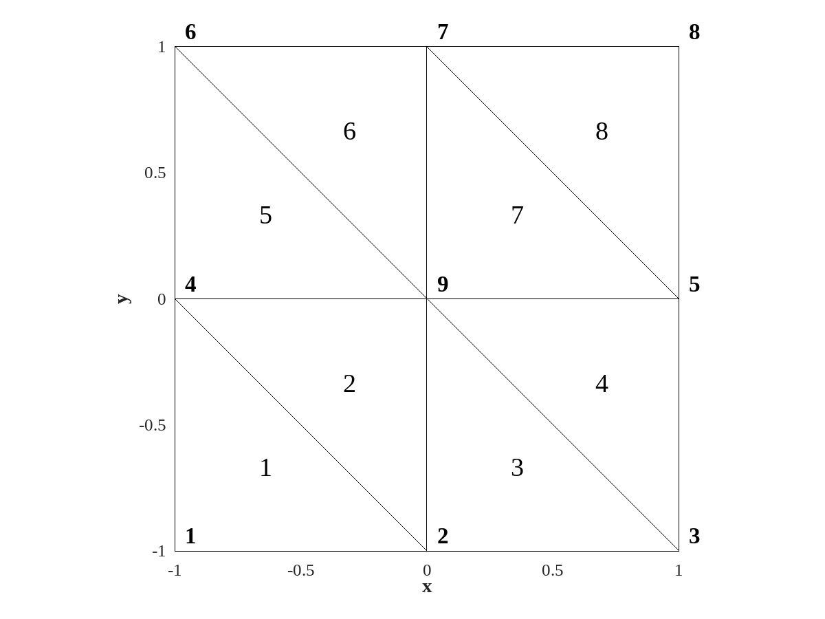
Figure 4.5: A simple $3\times 3$ grid. Nodes are numbered with a bold font and element numbers are show in large characters.

There are $M=9$ nodes, of which $D=8$ are at the boundaries We shall need the stiffness matrix $\mathcal{K}$ . Following

Element Matrices

The one-dimensional stiffness matrix is defined in equation 1.23. In two dimensions we use Maxima to find the elements of $\mathcal{K}e$ are:

Ke_{mn}=\int_{A}\!\left(\frac{\partial\phi_{m}}{\partial x}\frac{\partial\phi_% {n}}{\partial x}+\frac{\partial\phi_{m}}{\partial y}\frac{\partial\phi_{n}}{% \partial x}\right)\,da=A\begin{bmatrix}2&-1&-1\\ -1&1&0\\ -1&0&1\end{bmatrix}

(4.29)

where $A$ is the area of the test function.

Global Matrices

The assembly of $\mathcal{K}$ after the contributions from elements 1 and 2 is as follows:

\mathcal{K}=A\begin{bmatrix}2&-1&0&-1&0&0&0&0&0\\ -1&1&0&0&0&0&0&0&0\\ 0&0&0&0&0&0&0&0&0\\ -1&0&0&1&0&0&0&0&0\\ 0&0&0&0&0&0&0&0&0\\ 0&0&0&0&0&0&0&0&0\\ 0&0&0&0&0&0&0&0&0\\ 0&0&0&0&0&0&0&0&0\\ 0&0&0&0&0&0&0&0&0\\ \end{bmatrix};\quad A\begin{bmatrix}2&-1&0&-1&0&0&0&0&0\\ -1&2&0&0&0&0&0&0&-1\\ 0&0&0&0&0&0&0&0&0\\ -1&0&0&2&0&0&0&0&-1\\ 0&0&0&0&0&0&0&0&0\\ 0&0&0&0&0&0&0&0&0\\ 0&0&0&0&0&0&0&0&0\\ 0&0&0&0&0&0&0&0&0\\ 0&-1&0&-1&0&0&0&0&2\\ \end{bmatrix}.

(4.30)

It is useful to notice that after contribution from the second element have been added in, the bottom line of $\mathcal{K}$ is no longer zero. This is because element $2$ includes element $9$ as one ot the vertices, corresponding to the last row of $\mathcal{K}$ . After adding in the six other elements, $\mathcal{K}$ becomes:

\mathcal{K}=\frac{1}{2}\begin{bmatrix}2&-1&0&-1&0&0&0&0&0\\ -1&4&-1&0&0&0&0&0&-2\\ 0&-1&2&0&-1&0&0&0&0\\ -1&0&0&4&0&-1&0&0&-2\\ 0&0&-1&0&4&0&0&-1&-2\\ 0&0&0&-1&0&2&-1&0&0\\ 0&0&0&0&0&-1&4&-1&-2\\ 0&0&0&0&-1&0&-1&2&0\\ 0&-2&0&-2&-2&0&-2&0&8\\ \end{bmatrix}.

(4.31)

The top 8 rows of $\mathcal{K}$ are to be ignored. The last row shows that the value at the unknown node $9$ is equal to the average of the values at nodes $2$ , $4$ , $5$ and $7$ . This is the classic five-point Laplacian. The solution is $\psi_{9}=\psi_{4}=\psi_{6}=0$ .

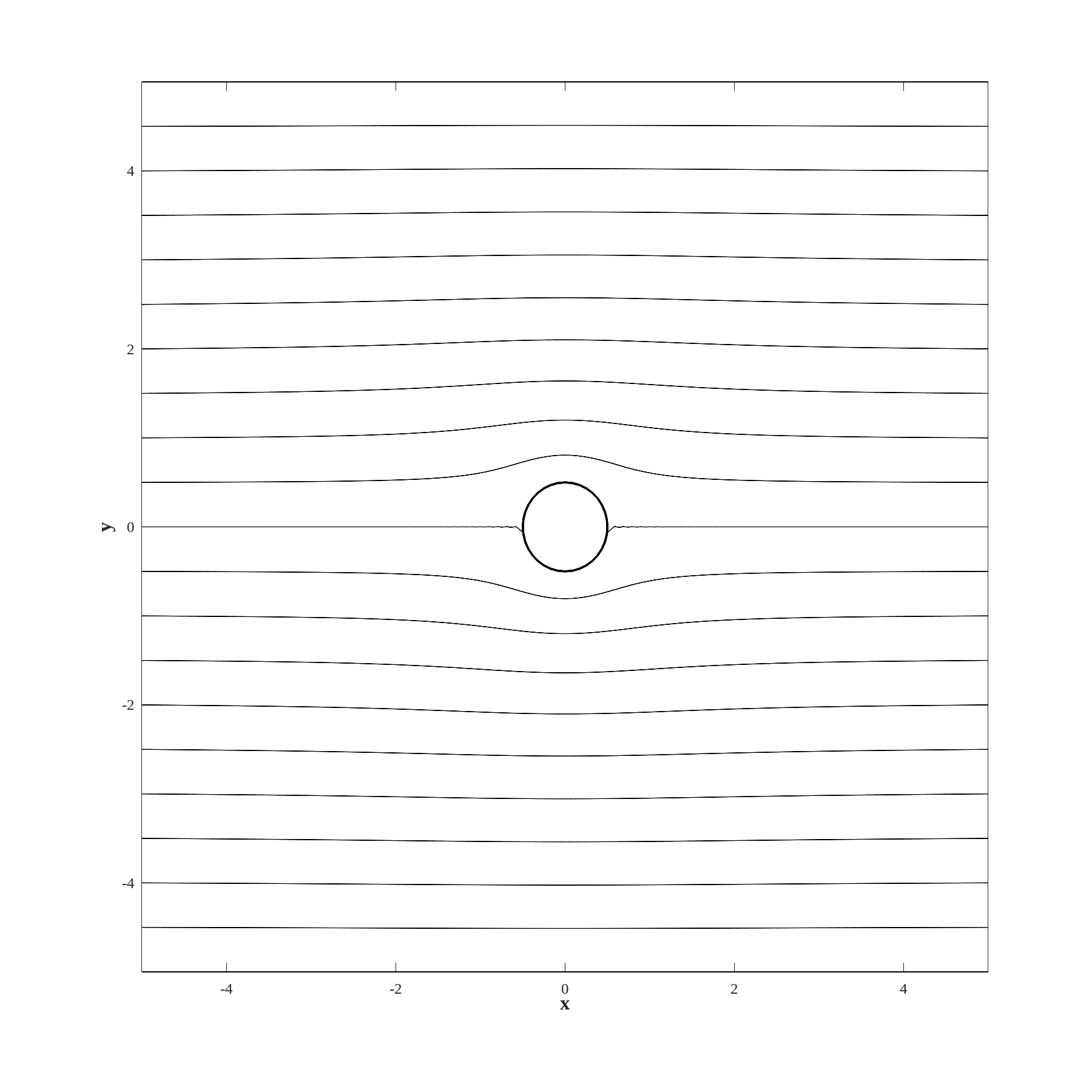
To evaluate the streamlines for fluid flowing over a cylinder, we use grid illustrated in the center of figure LABEL:Fi:C4S3figure1. We need to specify the streamfunction on all boundaries, including the cylinder, where we take the streamfunction to be zero. The solution, obtained with script LABEL:sec:OctaveC4S4figure6 is illustrated in figure 4.6.

Streamlines obtained with
script — Figure 4.6: Streamlines obtained with script 4.5.2 for flow around a circle of diameter $1$ . The contour line interval is $1/2$ . The grid includes 11572 nodes.

4.4 The Potential Function

The potential function $\varphi$ still solves Laplace’s equation but the boundary conditions are Neumann conditions on the normal gradient at a boundary:

\nabla^{2}\varphi=0;\quad\frac{\partial\varphi}{\partial n}=0\;\mbox{on all % boundaries except}\;\frac{\partial\varphi}{\partial x}=1\;\mbox{on}\;x=\pm x_{% max}.

(4.32)

4.4.1 Weak Form

The weak form is still given by equation 4.25, however the right hand side of that equations can no longer be neglected along all the boundaries. At solid boundaries (top and bottom of channel and cylinder), the normal gradient is zero, so there is no contribution. Along the right and left boundaries, the right hand term must be taken into account.

The matrix form for the potential flow problem is

\mathcal{K}\bm{\varphi}=\bm{F}\quad\mbox{where}\quad\bm{F}=\int_{S}\,\phi_{m}ds

(4.33)

Contribution to the boundary forcing $\bm{F}$ are due to the nonhomogeneous Neumann boundary conditions along the right and left boundaries. Because linear TF are used in the interior, the test functions $\phi_{m}^{1d}$ along the edge are straight lines, and their average height is always $1/2$ . Along the edge, these TFs are the same as illustrated in figure 1.4. The base of the test function for the first and last nodes is half that of the other boundary TF. The boundary contributions are therefore:

\bm{F}_{x=1}=\begin{bmatrix}x(E(2),2)-x(E(1),2)\\ x(E(3),2)-x(E(1),2)\\ \vdots\\ x(E(nE),2)-x(E(nE-2),2)\\ x(E(nE),2)-x(E(nE-1),2)\end{bmatrix}

(4.34)

where $x(E,2)$ are the ordinates of all nodes along the right (East, $x=1$ ) boundary. The boundary forcing term for the left side of the grid is minus the right side boundary forcing, since $\partial\varphi/\partial n=-1$ along the left boundary.

Attempts to solve the system 4.33 run into the further difficulty that there is no information about the mean value of $\varphi$ . Because of this the matrix $\mathcal{K}$ is singular. The way around this is to augment the system 4.32 by adding a constraint that the mean value of $\phi$ is some known value, equal to zero. This leads to an augmented matrix system:

\begin{bmatrix}K_{1,1}&K_{1,2}&\cdots&\cdots&K_{1,M-1}&K_{1,M}&1\\ K_{2,1}&K_{2,2}&\cdots&\cdots&K_{2,M-1}&K_{2,M}&1\\ \vdots&\ddots&\ddots&\ddots&\vdots&\vdots&\vdots\\ K_{M-1,1}&K_{M-1,2}&\cdots&\cdots&K_{M-1,M-1}&K_{M-1,M}&1\\ K_{M,1}&K_{M,2}&\cdots&\cdots&K_{M,M-1}&K_{M,M}&1\\ 1&1&\cdots&\cdots&1&1&0\end{bmatrix}\begin{bmatrix}\varphi_{1}\\ \varphi_{2}\\ \vdots\\ \varphi_{M-1}\\ \varphi_{M}\\ \lambda\end{bmatrix}=\begin{bmatrix}F_{1}\\ F_{2}\\ \vdots\\ F_{M-1}\\ F_{M}\\ 0\end{bmatrix}

(4.35)

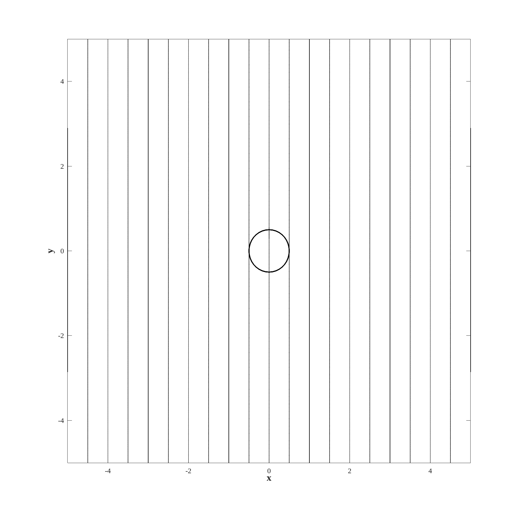
The potemtial function derived by solving the linear system 4.35 is illustrated in figure 4.7. The grid is the same as the used to produce figure LABEL:Fi:C4S4figure6.

Figure 4.7: Potential function $\varphi$ . lines of constant potential are normal an any location to the strealines illustrated in figure LABEL:Fi:C4S4figure6. The contour line interval is $1/2$ . The grid includes 11572 nodes.

Exercises

1.

Reproduce figure 4.6 for an ellipse at some non-zero angle of attack, and the NACA airfoil described in Persson’s website.

4.5 Scripts

4.5.1 Octave: Three DistMesh Grids

⬇

clear;

%%ID Chap 4 Sec 2 3 grids drawn with distmesh

%% Laplaces equation in FEM is -K*soln=Force

%% requires distmesh be installed in path

%% requires ShowMesh.m

hmin=0.1;% very few values work. was hmin=1

xmin=-1.5;xmax=1.5;ymin=-1;ymax=1;

pfix=[xmin,ymin;xmin,ymax;xmax,ymin;xmax,ymax];% fixed node positions

bbox=[xmin,ymin;xmax,ymax];%% LL and UR corners of bounding box

%% function that returns distance from point p to rectangle xmin,xmax,ymin,ymax

fd=inline(”drectangle(p,xmin,xmax,ymin,ymax)”,”p”);

[xp,tp]␣=␣distmesh2d(fd,␣@huniform,␣hmin,␣bbox,␣pfix);

np=length(xp(:,1));ne=length(tp(:,1));

set(gcf,’position’,[10,1000,1500,400]);clf;

axes(’position’,[0.03,0.075,0.3,0.8]);

ShowMesh(xp,tp);title(’Rectangular␣Grid’,’fontsize’,14);

radius=0.25;

fd=inline(”ddiff(drectangle(p,xmin,xmax,ymin,ymax),dcircle(p,0,0,radius))”,”p”);

[xp,tp]␣=␣distmesh2d(fd,␣@huniform,␣hmin,␣bbox,␣pfix);

axes(’position’,[0.36,0.075,0.3,0.8]);

ShowMesh(xp,tp);title(’Circle␣Inside␣Rectangular␣Grid’,’fontsize’,14);

maxh=4;

fh=inline(”min(2*sqrt(sum(p.^2,2))/radius-1,maxh)”,”p”);%

hmininit=0.025;

[xp,tp]=distmesh2d(fd,fh,hmininit,bbox,pfix);

axes(’position’,[0.69,0.075,0.3,0.8]);

ShowMesh(xp,tp);title(’Refined␣Grid␣Near␣Cylinder’,’fontsize’,14);

set(gcf,’paperpositionmode’,’manual’,’paperposition’,[0.25␣0.25␣15␣4])

print␣-dpng␣../../words/figs/C4/C4S2figure1.png

4.5.2 Octave: Stream Function

⬇

clear;

%%ID Chap 4 Sec 3 del^2 psi=0, flow around cylinder;

%%ID Dirichlet BC on all boundaries

%% Make a Grid

hmin=0.1;

xmin=-5;xmax=5;ymin=-5;ymax=5;

pfix=[xmin,ymin;xmin,ymax;xmax,ymin;xmax,ymax];% fixed node positions

bbox=[xmin,ymin;xmax,ymax];%% LL and UR corners of bounding box

radius=0.5;

fd=inline(”ddiff(drectangle(p,xmin,xmax,ymin,ymax),dcircle(p,0,0,radius))”,”p”);

[xp,tp]␣=␣distmesh2d(fd,␣@huniform,␣hmin,␣bbox,␣pfix);

np=length(xp(:,1));nelement=length(tp(:,1));

%%␣locate␣boundaries

smallno=1e-8;%␣any␣smaller␣makes␣trouble

N=find(xp(:,2)>ymax-smallno);[~,order]=sort(xp(N,1));N=N(order);

S=find(xp(:,2)<ymin+smallno);[~,order]=sort(xp(S,1));S=S(order);

W=find(xp(:,1)<smallno+xmin);[~,order]=sort(xp(W,2));W=W(order);nW=length(W);

E=find(xp(:,1)>xmax-smallno);[~,order]=sort(xp(E,2));E=E(order);nE=length(E);

bndedges=boundedges(xp,tp);bndnodes=[bndedges(:,1);bndedges(end,2)];%␣all␣bnd

bndnodes=[bndedges(:,1);bndedges(end,2)];

%%␣Assemble␣Global␣matrix␣K␣element␣by␣element

%%␣Linear␣TF

K=sparse(np,np);␣%%␣initialize

for␣ke=1:nelement

␣␣nodes=tp(ke,:);

␣␣T=[ones(3,1),xp(nodes,:)];

␣␣Area=abs(det(T))/2;

␣␣C=inv(T);

␣␣grad=C(2:3,:);

␣␣Ke=Area*transpose(grad)*grad;%␣stiffness␣contribution

␣␣K(nodes,nodes)=K(nodes,nodes)+Ke;

end

%%␣set␣Dirichlet␣BC

outnodes=unique([N;W;S;E]);psi=zeros(np,1);psi(outnodes)=xp(outnodes,2);

cylnodes=setdiff(bndnodes,outnodes);psi(cylnodes)=0;

Dirichlet=[outnodes;cylnodes];

Interior=setdiff([1:np]’,Dirichlet);

tildeK=K(Interior,Interior);

hatK=K(Interior,Dirichlet);

psi(Interior)=tildeK\(-hatK*psi(Dirichlet));

%%␣Plot

set(gcf,’position’,[10,1000,1200,1200]);clf;

minpsi=-5;maxpsi=5;incpsi=0.5;

tricontour(tp,␣xp(:,1),xp(:,2),␣psi,␣[minpsi:incpsi:maxpsi],’k’);hold␣on

%tricontour(tp,␣xp(:,1),xp(:,2),␣psi,␣[0␣0],’k’);

%%␣show␣cylinder

theta=linspace(0,2*pi,37);

plot(cos(theta)/2,sin(theta)/2,’k’,’linewidth’,2);␣%␣radius␣is␣1/2

xlabel(’x’,’fontsize’,16,’fontweight’,’bold’);

ylabel(’y’,’fontsize’,16,’fontweight’,’bold’);

axis([-5,5,-5,5])

set(gcf,’paperpositionmode’,’manual’,’paperposition’,[0.25␣0.25␣12␣12])

print␣-dpng␣../../words/figs/C4/C4S3figure6.png

4.5.3 Octave: Potential Function

⬇

%%ID Chap 4 Sec 3 del^2 varphi=0, flow around cylinder;

%%ID Neumann BC on all bnd, with constraint

%% Make a Grid

hmin=0.1;

xmin=-5;xmax=5;ymin=-5;ymax=5;

pfix=[xmin,ymin;xmin,ymax;xmax,ymin;xmax,ymax];% fixed node positions

bbox=[xmin,ymin;xmax,ymax];%% LL and UR corners of bounding box

radius=0.5;

fd=inline(”ddiff(drectangle(p,xmin,xmax,ymin,ymax),dcircle(p,0,0,radius))”,”p”);

[xp,tp]␣=␣distmesh2d(fd,␣@huniform,␣hmin,␣bbox,␣pfix);

np=length(xp(:,1));nelement=length(tp(:,1));

%%␣locate␣boundaries

smallno=1e-8;%␣any␣smaller␣makes␣trouble

N=find(xp(:,2)>ymax-smallno);[~,order]=sort(xp(N,1));N=N(order);

S=find(xp(:,2)<ymin+smallno);[~,order]=sort(xp(S,1));S=S(order);

W=find(xp(:,1)<smallno+xmin);[~,order]=sort(xp(W,2));W=W(order);nW=length(W);

E=find(xp(:,1)>xmax-smallno);[~,order]=sort(xp(E,2));E=E(order);nE=length(E);

%%␣Assemble␣Global␣matrix␣K␣element␣by␣element

%%␣Linear␣TF

K=sparse(np,np);

for␣ke=1:nelement

␣␣nodes=tp(ke,:);

␣␣T=[ones(3,1),xp(nodes,:)];

␣␣Area=abs(det(T))/2;

␣␣C=inv(T);

␣␣grad=C(2:3,:);

␣␣Ke=Area*transpose(grad)*grad;

␣␣K(nodes,nodes)=K(nodes,nodes)+Ke;

end

%%␣augment␣K

K=[K,ones(np,1);ones(1,np),0];

Force=zeros(np,1);

%%␣minus␣sign␣on␣west␣side␣because␣integration␣path␣in␣reverse

Force(W(1))=-(xp(W(2),2)-xp(W(1),2));%␣delta␣y␣for␣1st␣node␣on␣L

Force(W(nW))=-(xp(W(nW),2)-xp(W(nW-1),2));%␣delta␣y

Force(W(2:nW-1))=-(xp(W(3:nW),2)-xp(W(1:nW-2),2));%␣delta␣y␣btwn␣ends

Force(E(1))=xp(E(2),2)-xp(E(1),2);%␣delta␣y␣for␣1st␣node␣on␣R

Force(E(nE))=xp(E(nE),2)-xp(E(nE-1),2);%

Force(E(2:nE-1))=xp(E(3:nE),2)-xp(E(1:nE-2),2);%

Force=Force/2;%␣because␣the␣average␣height␣of␣each␣triangular␣element␣is␣1/2

Force=[Force;0];

varphi=K\Force;varphi(np+1)

set(gcf,’position’,[10,1000,1200,1200]);clf;

minvarphi=min(varphi);maxvarphi=max(varphi);rngvarphi=maxvarphi-minvarphi;nclines=11;

tricontour(tp,␣xp(:,1),xp(:,2),␣varphi,␣[-5:0.5:5],’k’);hold␣on

tricontour(tp,␣xp(:,1),xp(:,2),␣varphi,␣[0␣0],’k’);

theta=linspace(0,2*pi,37);plot(cos(theta)/2,sin(theta)/2,’k’,’linewidth’,2);%␣cylinder

xlabel(’x’,’fontsize’,16,’fontweight’,’bold’);

ylabel(’y’,’fontsize’,16,’fontweight’,’bold’);

axis([-5,5,-5,5])

set(gcf,’paperpositionmode’,’manual’,’paperposition’,[0.25␣0.25␣12␣12])

print␣-dpng␣../../words/figs/C4/C4S4figure7.png